## The basic files and libraries needed for most presentations
# creates the libraries and common-functions sections
read_chunk("../common/utility_functions.R")require(ggplot2) #for plots
require(lattice) # nicer scatter plots
require(plyr) # for processing data.frames
library(dplyr)
require(grid) # contains the arrow function
require(jpeg)
require(doMC) # for parallel code
require(png) # for reading png images
require(gridExtra)
require(reshape2) # for the melt function
#if (!require("biOps")) {
# # for basic image processing
# devtools::install_github("cran/biOps")
# library("biOps")
#}
## To install EBImage
if (!require("EBImage")) { # for more image processing
source("http://bioconductor.org/biocLite.R")
biocLite("EBImage")
}
used.libraries<-c("ggplot2","lattice","plyr","reshape2","grid","gridExtra","biOps","png","EBImage")# start parallel environment
registerDoMC()
# functions for converting images back and forth
im.to.df<-function(in.img,out.col="val") {
out.im<-expand.grid(x=1:nrow(in.img),y=1:ncol(in.img))
out.im[,out.col]<-as.vector(in.img)
out.im
}
df.to.im<-function(in.df,val.col="val",inv=F) {
in.vals<-in.df[[val.col]]
if(class(in.vals[1])=="logical") in.vals<-as.integer(in.vals*255)
if(inv) in.vals<-255-in.vals
out.mat<-matrix(in.vals,nrow=length(unique(in.df$x)),byrow=F)
attr(out.mat,"type")<-"grey"
out.mat
}
ddply.cutcols<-function(...,cols=1) {
# run standard ddply command
cur.table<-ddply(...)
cutlabel.fixer<-function(oVal) {
sapply(oVal,function(x) {
cnv<-as.character(x)
mean(as.numeric(strsplit(substr(cnv,2,nchar(cnv)-1),",")[[1]]))
})
}
cutname.fixer<-function(c.str) {
s.str<-strsplit(c.str,"(",fixed=T)[[1]]
t.str<-strsplit(paste(s.str[c(2:length(s.str))],collapse="("),",")[[1]]
paste(t.str[c(1:length(t.str)-1)],collapse=",")
}
for(i in c(1:cols)) {
cur.table[,i]<-cutlabel.fixer(cur.table[,i])
names(cur.table)[i]<-cutname.fixer(names(cur.table)[i])
}
cur.table
}
# since biOps isn't available use a EBImage based version
imgSobel<-function(img) {
kern<-makeBrush(3)*(-1)
kern[2,2]<-8
filter2(img,kern)
}
show.pngs.as.grid<-function(file.list,title.fun,zoom=1) {
preparePng<-function(x) rasterGrob(readPNG(x,native=T,info=T),width=unit(zoom,"npc"),interp=F)
labelPng<-function(x,title="junk") (qplot(1:300, 1:300, geom="blank",xlab=NULL,ylab=NULL,asp=1)+
annotation_custom(preparePng(x))+
labs(title=title)+theme_bw(24)+
theme(axis.text.x = element_blank(),
axis.text.y = element_blank()))
imgList<-llply(file.list,function(x) labelPng(x,title.fun(x)) )
do.call(grid.arrange,imgList)
}
## Standard image processing tools which I use for visualizing the examples in the script
commean.fun<-function(in.df) {
ddply(in.df,.(val), function(c.cell) {
weight.sum<-sum(c.cell$weight)
data.frame(xv=mean(c.cell$x),
yv=mean(c.cell$y),
xm=with(c.cell,sum(x*weight)/weight.sum),
ym=with(c.cell,sum(y*weight)/weight.sum)
)
})
}
colMeans.df<-function(x,...) as.data.frame(t(colMeans(x,...)))
pca.fun<-function(in.df) {
ddply(in.df,.(val), function(c.cell) {
c.cell.cov<-cov(c.cell[,c("x","y")])
c.cell.eigen<-eigen(c.cell.cov)
c.cell.mean<-colMeans.df(c.cell[,c("x","y")])
out.df<-cbind(c.cell.mean,
data.frame(vx=c.cell.eigen$vectors[1,],
vy=c.cell.eigen$vectors[2,],
vw=sqrt(c.cell.eigen$values),
th.off=atan2(c.cell.eigen$vectors[2,],c.cell.eigen$vectors[1,]))
)
})
}
vec.to.ellipse<-function(pca.df) {
ddply(pca.df,.(val),function(cur.pca) {
# assume there are two vectors now
create.ellipse.points(x.off=cur.pca[1,"x"],y.off=cur.pca[1,"y"],
b=sqrt(5)*cur.pca[1,"vw"],a=sqrt(5)*cur.pca[2,"vw"],
th.off=pi/2-atan2(cur.pca[1,"vy"],cur.pca[1,"vx"]),
x.cent=cur.pca[1,"x"],y.cent=cur.pca[1,"y"])
})
}
# test function for ellipse generation
# ggplot(ldply(seq(-pi,pi,length.out=100),function(th) create.ellipse.points(a=1,b=2,th.off=th,th.val=th)),aes(x=x,y=y))+geom_path()+facet_wrap(~th.val)+coord_equal()
create.ellipse.points<-function(x.off=0,y.off=0,a=1,b=NULL,th.off=0,th.max=2*pi,pts=36,...) {
if (is.null(b)) b<-a
th<-seq(0,th.max,length.out=pts)
data.frame(x=a*cos(th.off)*cos(th)+b*sin(th.off)*sin(th)+x.off,
y=-1*a*sin(th.off)*cos(th)+b*cos(th.off)*sin(th)+y.off,
id=as.factor(paste(x.off,y.off,a,b,th.off,pts,sep=":")),...)
}
deform.ellipse.draw<-function(c.box) {
create.ellipse.points(x.off=c.box$x[1],
y.off=c.box$y[1],
a=c.box$a[1],
b=c.box$b[1],
th.off=c.box$th[1],
col=c.box$col[1])
}
bbox.fun<-function(in.df) {
ddply(in.df,.(val), function(c.cell) {
c.cell.mean<-colMeans.df(c.cell[,c("x","y")])
xmn<-emin(c.cell$x)
xmx<-emax(c.cell$x)
ymn<-emin(c.cell$y)
ymx<-emax(c.cell$y)
out.df<-cbind(c.cell.mean,
data.frame(xi=c(xmn,xmn,xmx,xmx,xmn),
yi=c(ymn,ymx,ymx,ymn,ymn),
xw=xmx-xmn,
yw=ymx-ymn
))
})
}
# since the edge of the pixel is 0.5 away from the middle of the pixel
emin<-function(...) min(...)-0.5
emax<-function(...) max(...)+0.5
extents.fun<-function(in.df) {
ddply(in.df,.(val), function(c.cell) {
c.cell.mean<-colMeans.df(c.cell[,c("x","y")])
out.df<-cbind(c.cell.mean,data.frame(xmin=c(c.cell.mean$x,emin(c.cell$x)),
xmax=c(c.cell.mean$x,emax(c.cell$x)),
ymin=c(emin(c.cell$y),c.cell.mean$y),
ymax=c(emax(c.cell$y),c.cell.mean$y)))
})
}
common.image.path<-"../common"
qbi.file<-function(file.name) file.path(common.image.path,"figures",file.name)
qbi.data<-function(file.name) file.path(common.image.path,"data",file.name)
th_fillmap.fn<-function(max.val) scale_fill_gradientn(colours=rainbow(10),limits=c(0,max.val))Quantitative Big Imaging
author: Kevin Mader date: 10 March 2016 width: 1440 height: 900 css: ../common/template.css transition: rotate
Basic Segmentation and Discrete Binary Structures
Course Outline
source('../common/schedule.R')- 25th February - Introduction and Workflows
- 3rd March - Image Enhancement (A. Kaestner)
- 10th March - Basic Segmentation, Discrete Binary Structures
- 17th March - Advanced Segmentation
- 24th March - Analyzing Single Objects
- 7th April - Analyzing Complex Objects
- 14th April - Spatial Distribution
- 21st April - Statistics and Reproducibility
- 28th April - Dynamic Experiments
- 12th May - Scaling Up / Big Data
- 19th May - Guest Lecture - High Content Screening
- 26th May - Guest Lecture - Machine Learning / Deep Learning and More Advanced Approaches
- 2nd June - Project Presentations
Lesson Outline
- Motivation
- Qualitative Approaches
- Thresholding
- Other types of images
- Selecting a good threshold
- Implementation
- Morphology
- Contouring / Mask Creation
Applications
- Simple two-phase materials (bone, cells, etc)
- Beyond 1 channel of depth
- Multiple phase materials
- Filling holes in materials
- Segmenting Fossils
- Attempting to segment the cortex in brain imaging

Literature / Useful References
- Jean Claude, Morphometry with R
- Online through ETHZ
- Buy it
- John C. Russ, “The Image Processing Handbook”,(Boca Raton, CRC Press)
- Available online within domain ethz.ch (or proxy.ethz.ch / public VPN)
Models / ROC Curves
Motivation: Why do we do imaging experiments?
incremental: true
- Exploratory
- To visually, qualitatively examine samples and differences between them
- No prior knowledge or expectations
- To test a hypothesis
- Quantitative assessment coupled with statistical analysis
- Does temperature affect bubble size?
- Is this gene important for cell shape and thus mechanosensation in bone?
- Does higher canal volume make bones weaker?
- Does the granule shape affect battery life expectancy?
- What we are looking at

- What we get from the imaging modality
dkimg<-jpeg::readJPEG("../common/figures/Average_prokaryote_cell.jpg")
material.img<-1-(dkimg[,,1]+dkimg[,,2]+dkimg[,,3])/3
# assume the sample is constant 0.1m thick and color indicates alpha
gray.img<-1.0*exp(-material.img*0.1)
cellImage<-im.to.df(gray.img)
ggplot(cellImage,aes(x=y,y=-x,fill=val))+
  geom_tile()+guides(fill=F)+theme_bw(20)
To test a hypothesis
- We perform an experiment bone to see how big the cells are inside the tissue
↓

2560 x 2560 x 2160 x 32 bit = 56GB / sample
- Filtering and Preprocessing!
↓ - 20h of computer time later …
- 56GB of less noisy data
- Way too much data, we need to reduce
What did we want in the first place
incremental: true
Single number:
- volume fraction,
- cell count,
- average cell stretch,
- cell volume variability
Why do we perform segmentation?
- In model-based analysis every step we peform, simple or complicated is related to an underlying model of the system we are dealing with
- Occam’s Razor is very important here : The simplest solution is usually the right one
- Bayesian, neural networks optimized using genetic algorithms with Fuzzy logic has a much larger parameter space to explore, establish sensitivity in, and must perform much better and be tested much more thoroughly than thresholding to be justified.
- We will cover some of these techniques in the next 2 lectures since they can be very powerful particularly with unknown data
Review: Filtering and Image Enhancement
incremental: true
- This was a noise process which was added to otherwise clean imaging data
Imeasured(x, y)=Isample(x, y)+Noise(x, y)- What would the perfect filter be
Filter * Isample(x, y)=Isample(x, y)
Filter * Noise(x, y)=0
Filter∗Imeasured(x,y)=Filter∗Ireal(x,y)+Filter∗Noise(x,y)→Isample(x,y)- What most filters end up doing
Filter * Imeasured(x, y)=90%Ireal(x, y)+10%Noise(x, y) - What bad filters do
Filter * Imeasured(x, y)=10%Ireal(x, y)+90%Noise(x, y)
Qualitative Metrics: What did people used to do?
- What comes out of our detector / enhancement process
ggplot(cellImage,aes(x=y,y=400-x,fill=val))+
  geom_tile()+guides(fill=F)+theme_bw(20)+labs(x="x",y="y")
- Identify objects by eye
- Count, describe qualitatively: “many little cilia on surface”, “long curly flaggelum”, “elongated nuclear structure”
- Morphometrics
- Trace the outline of the object (or sub-structures)
- Can calculate the area by using equal-weight-paper
- Employing the “cut-and-weigh” method
Segmentation Approaches
They match up well to the world view / perspective

Model-Based
- → Experimentalist
- Problem-driven
- Top-down
- Reality Model-based
Machine Learning Approach
- → Computer Vision / Deep Learning
- Results-driven
Model-based Analysis

- Many different imaging modalities ( μCT to MRI to Confocal to Light-field to AFM).
- Similarities in underlying equations
- different coefficients, units, and mechanism
Imeasured(→x)=Fsystem(Istimulus(→x),Ssample(→x))
Direct Imaging (simple)
- Fsystem(a, b)=a * b
- Istimulus = Beamprofile
- $S_{system} = \alpha(\vec{x})$
$\longrightarrow \alpha(\vec{x})=\frac{I_{measured}(\vec{x})}{\textrm{Beam}_{profile}(\vec{x})}$
grad.beam.profile<-matrix(rep(0.9+0.00*c(1:nrow(gray.img)),ncol(gray.img)),dim(gray.img))
sample.img<-1.0*exp(-material.img*0.1)
ccd.img<-sample.img * grad.beam.profile
model.image<-subset(
  rbind(
  cbind(im.to.df(grad.beam.profile),type="Beam"),
  cbind(im.to.df(sample.img),type="Sample"),
  cbind(im.to.df(ccd.img),type="Detector")
  ),
  x%%3==0 & y%%3==0 # downsample by 9
  )
ggplot(model.image,aes(x=y,y=x,fill=val))+
  geom_tile()+
  guides(fill=F)+
  facet_grid(type~.)+
  coord_equal()+
  theme_bw(20)
Nonuniform Beam-Profiles
In many setups there is un-even illumination caused by incorrectly adjusted equipment and fluctations in power and setups
grad.beam.profile<-matrix(rep(0.9+0.001*c(1:nrow(gray.img)),ncol(gray.img)),dim(gray.img))
sample.img<-1.0*exp(-material.img*0.1)
ccd.img<-sample.img * grad.beam.profile
model.image<-subset(
  rbind(
  cbind(im.to.df(grad.beam.profile),type="Beam"),
  cbind(im.to.df(sample.img),type="Sample"),
  cbind(im.to.df(ccd.img),type="Detector")
  ),
  x%%3==0 & y%%3==0 # downsample by 9
  )
ggplot(model.image,aes(x=y,y=x,fill=val))+
  geom_tile()+
  facet_grid(type~.)+
  coord_equal()+
  labs(fill="")+
  scale_fill_gradientn(colours=rainbow(6))+
  theme_bw(20)
Frequently there is a fall-off of the beam away from the center (as is the case of a Gaussian beam which frequently shows up for laser systems). This can make extracting detail away from the center challenging
beam.profile<-mutate(
  expand.grid(x=1:nrow(material.img),y=1:ncol(material.img)),
  val=exp(-((x-mean(x))^2+(y-mean(y))^2)/350^2) # just a simple gaussian profile
  )
beam.profile<-df.to.im(beam.profile)
sample.img<-1.0*exp(-material.img*0.1)
ccd.img<-sample.img * beam.profile
model.image<-subset(
  rbind(
  cbind(im.to.df(beam.profile),type="Beam"),
  cbind(im.to.df(sample.img),type="Sample"),
  cbind(im.to.df(ccd.img),type="Detector")
  ),
  x%%3==0 & y%%3==0 # downsample by 9
  )
ggplot(model.image,aes(x=y,y=x,fill=val))+
  geom_tile()+
  facet_grid(type~.)+
  coord_equal()+
  scale_fill_gradientn(colours=rainbow(6))+
  labs(fill="")+
  theme_bw(20)
Absorption Imaging (X-ray, Ultrasound, Optical)
- For absorption/attenuation imaging → Beer-Lambert Law
Idetector=Isource⏟Istimulusexp(−αd)⏟Ssample Different components have a different α based on the strength of the interaction between the light and the chemical / nuclear structure of the material
Isample(x, y)=Isourceexp(−α(x, y)d)
α = f(N, Z, σ, ⋯)- For segmentation this model is:
- there are 2 (or more) distinct components that make up the image
these components are distinguishable by their values (or vectors, colors, tensors, …)
nx<-4
ny<-4
grad.im<-expand.grid(x=c(-nx:nx)/nx*2*pi,y=c(-ny:ny)/ny*2*pi)
phase.im<-runif(nrow(grad.im))
grad.im<-cbind(grad.im,
               col=1*(phase.im>0.66)+
                 2*(phase.im<0.33)+
                 0.4*runif(nrow(grad.im),min=-1,max=1))
bn.wid<-diff(range(grad.im$col))/10

bl.fun<-function(x) 1*exp(-x*0.5)

ggplot(grad.im,aes(x=col,y=bl.fun(col)))+
  geom_point(aes(color=cut_interval(col,3)))+
  geom_segment(data=data.frame(
    x=c(0.5,1.5),y=c(0.25),
    xend=c(0.5,1.5),yend=c(1.25)
    ),aes(x=x,y=y,xend=xend,yend=yend),size=3,alpha=0.5)+
  labs(x=expression(alpha(x,y)),y=expression(paste("I"[sample],"(x,y)")),title="Probability Density Function",fill="Groups")+theme_bw(20)
ggplot(grad.im,aes(x=col))+
  geom_density(aes(fill=cut_interval(col,3)))+
  geom_segment(data=data.frame(
    x=c(0.5,1.5),y=c(0),
    xend=c(0.5,1.5),yend=c(6)
    ),aes(x=x,y=y,xend=xend,yend=yend),
    size=3,alpha=0.5)+
  labs(x=expression(alpha(x,y)),y="Frequency",title="Probability Density Function",fill="Groups")+theme_bw(20)
Where does segmentation get us?
incremental: true
- We convert a decimal value (or something even more complicated like 3 values for RGB images, a spectrum for hyperspectral imaging, or a vector / tensor in a mechanical stress field)
to a single, discrete value (usually true or false, but for images with phases it would be each phase, e.g. bone, air, cellular tissue)
- 2560 x 2560 x 2160 x 32 bit = 56GB / sample
↓ 2560 x 2560 x 2160 x 1 bit = 1.75GB / sample
Applying a threshold to an image
Start out with a simple image of a cross with added noiseI(x, y)=f(x, y)
nx<-5
ny<-5
cross.im<-expand.grid(x=c(-nx:nx)/nx*2*pi,y=c(-ny:ny)/ny*2*pi)
cross.im<-cbind(cross.im,
               col=1.5*with(cross.im,abs(cos(x*y))/(abs(x*y)+(3*pi/nx)))+
                 0.5*runif(nrow(cross.im)))
bn.wid<-diff(range(cross.im$col))/10
ggplot(cross.im,aes(x=x,y=y,fill=col))+
  geom_tile()+
  scale_fill_gradient(low="black",high="white")+
  labs(fill="Intensity")+
  theme_bw(20)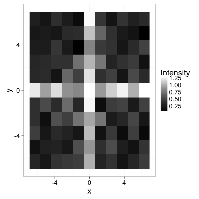
The intensity can be described with a probability density function
Pf(x, y)
ggplot(cross.im,aes(x=col))+geom_histogram(binwidth=bn.wid)+
  labs(x="Intensity",title="Probability Density Function")+
  theme_bw(20)
Applying a threshold to an image
By examining the image and probability distribution function, we can deduce that the underyling model is a whitish phase that makes up the cross and the darkish background
thresh.val<-0.75
cross.im$val<-(cross.im$col>=thresh.val)
ggplot(cross.im,aes(x=x,y=y))+
  geom_tile(aes(fill=col))+
  geom_tile(data=subset(cross.im,val),fill="red",color="black",alpha=0.3)+
  geom_tile(data=subset(cross.im,!val),fill="blue",color="black",alpha=0.3)+
  scale_fill_gradient(low="black",high="white")+
  labs(fill="Intensity")+
  theme_bw(20)
Applying the threshold is a deceptively simple operation
I(x,y)={1,f(x,y)≥0.50,f(x,y)<0.5
ggplot(cbind(cross.im,in.thresh=cross.im$col>=thresh.val),aes(x=col))+
  geom_histogram(binwidth=bn.wid,aes(fill=in.thresh))+
  labs(x="Intensity",color="In Threshold")+scale_fill_manual(values=c("blue","red"))+
  theme_bw(20)
Various Thresholds
thresh.vals<-c(2:10)/10
grad.im.th<-ldply(thresh.vals,function(thresh.val)
  cbind(cross.im,thresh=thresh.val,in.thresh=(cross.im$col>=thresh.val)))
ggplot(grad.im.th,aes(x=col))+
  geom_histogram(binwidth=bn.wid,aes(fill=in.thresh))+
  labs(x="Intensity",fill="Above Threshold")+facet_wrap(~thresh)+
  theme_bw(15)
ggplot(grad.im.th,aes(x=x,y=y))+
  geom_tile(aes(fill=in.thresh),color="black",alpha=0.75)+
  labs(fill="Above Threshold")+facet_wrap(~thresh)+
  theme_bw(20)
Segmenting Cells
cellImage<-im.to.df(jpeg::readJPEG("ext-figures/Cell_Colony.jpg"))
ggplot(cellImage,aes(x=x,y=y,fill=val))+
  geom_tile()+
  labs(fill="Intensity")+coord_equal()+
  theme_bw(20)

- We can peform the same sort of analysis with this image of cells
- This time we can derive the model from the basic physics of the system
- The field is illuminated by white light of nearly uniform brightness
- Cells absorb light causing darker regions to appear in the image
- Lighter regions have no cells
- Darker regions have cells
Different Threshold Values
th.vals<-seq(0.4,0.85,length.out=3)
thlabel<-function(x,...) switch(x,"Too low","Good","Too high")
im.vals<-ldply(1:length(th.vals),function(th.val)
  cbind(cellImage,
        in.thresh=ifelse(cellImage$val


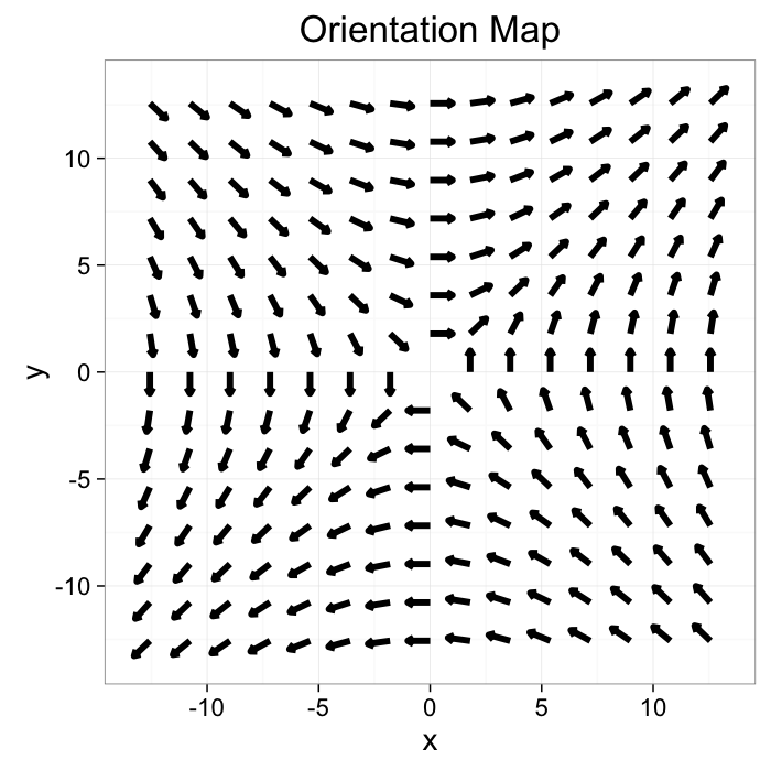
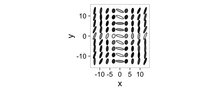
Other Image Types
While scalar images are easiest, it is possible for any type of image
$$ I(x,y) = \vec{f}(x,y) $$
nx<-7
ny<-7
n.pi<-4
grad.im<-expand.grid(x=c(-nx:nx)/nx*n.pi*pi,y=c(-ny:ny)/ny*n.pi*pi)
grad.im<-cbind(grad.im,
col=1.5*with(grad.im,abs(cos(x*y))/(abs(x*y)+(3*pi/nx)))+
0.5*runif(nrow(grad.im)),
x.vec=with(grad.im,y),
y.vec=with(grad.im,x))
# normalize vector
grad.im[,c("x.vec","y.vec")]<-with(grad.im,cbind(x.vec/(sqrt(x.vec^2+y.vec^2)),
y.vec/(sqrt(x.vec^2+y.vec^2))))
bn.wid<-c(diff(range(grad.im$x.vec))/10,diff(range(grad.im$y.vec))/10)
ggplot(grad.im,aes(x=x,y=y,fill=col))+
geom_segment(aes(xend=x+x.vec,yend=y+y.vec),arrow=arrow(length = unit(0.15,"cm")),size=2)+
scale_fill_gradient(low="black",high="white")+
guides(fill=F)+labs(title="Orientation Map")+
theme_bw(20)
The intensity can be described with two seperate or a single joint probability density function
$$ P_{\vec{f}\cdot \vec{i}}(x,y), P_{\vec{f}\cdot \vec{j}}(x,y) $$
ggplot(grad.im,aes(x=x.vec,y=y.vec))+
stat_bin2d(binwidth=c(0.25,.25),drop=F)+
labs(x="Pfx",y="Pfy",fill="Frequency",title="Orientation Histogram")+
xlim(-1,1)+ylim(-1,1)+
theme_bw(20)

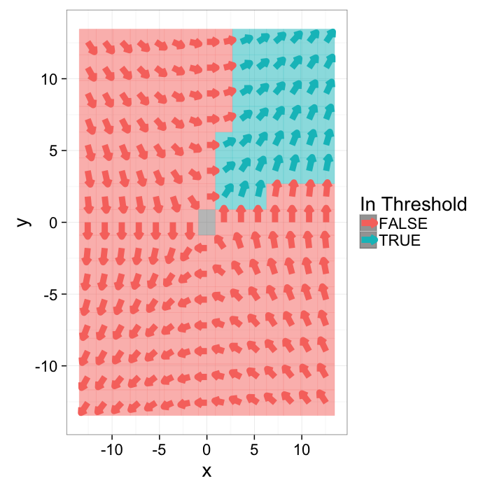
Applying a threshold
A threshold is now more difficult to apply since there are now two distinct variables to deal with. The standard approach can be applied to both
$$ I(x,y) =
\begin{cases}
1, & \vec{f}_x(x,y) \geq0.25 \text{ and}\\
& \vec{f}_y(x,y) \geq0.25 \\
0, & \text{otherwise}
\end{cases}$$
g.with.thresh<-cbind(grad.im,in.thresh=with(grad.im,x.vec>0.25 & y.vec>0.25))
ggplot(g.with.thresh,
aes(x=x,y=y,fill=in.thresh,color=in.thresh))+
geom_tile(alpha=0.5,aes(fill=in.thresh))+
geom_segment(aes(xend=x+x.vec,yend=y+y.vec),arrow=arrow(length = unit(0.2,"cm")),size=3)+
labs(color="In Threshold")+guides(fill=FALSE)+
theme_bw(20)
This can also be shown on the joint probability distribution as
bn.wid<-c(0.25,.25)
keep.bins<-expand.grid(x.vec=seq(-1,1,bn.wid[1]/10),y.vec=seq(-1,1,bn.wid[2]/10))
keep.bins<-cbind(keep.bins,in.thresh=with(keep.bins,x.vec>0.25 & y.vec>0.25))
ggplot(g.with.thresh,aes(x=x.vec,y=y.vec))+
stat_bin2d(binwidth=bn.wid,drop=F)+
geom_tile(data=subset(g.with.thresh,in.thresh),fill="red",alpha=0.4)+
labs(x="Pfx",y="Pfy",fill="Threshold")+xlim(-1,1)+ylim(-1,1)+
theme_bw(20)

Applying a threshold
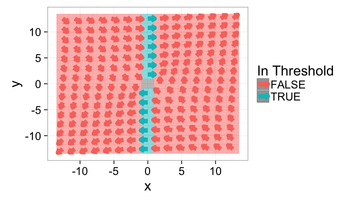
Given the presence of two variables; however, more advanced approaches can also be investigated. For example we can keep only components parallel to the x axis by using the dot product.
$$ I(x,y) =
\begin{cases}
1, & |\vec{f}(x,y)\cdot \vec{i}| = 1 \\
0, & \text{otherwise}
\end{cases}$$
i.vec<-c(1,0)
j.vec<-c(0,1)
g.cmp.thresh<-cbind(grad.im,in.thresh=with(grad.im,
abs(x.vec*i.vec[1]+y.vec*i.vec[2])==1
))
ggplot(g.cmp.thresh,
aes(x=x,y=y,fill=in.thresh,color=in.thresh))+
geom_tile(alpha=0.5,aes(fill=in.thresh))+
geom_segment(aes(xend=x+x.vec,yend=y+y.vec),arrow=arrow(length = unit(0.2,"cm")),size=3)+
labs(color="In Threshold")+guides(fill=FALSE)+
theme_bw(20)
Looking at Orientations
We can tune the angular acceptance by using the fact
$$\vec{x}\cdot\vec{y}=|\vec{x}| |\vec{y}| \cos(\theta_{x\rightarrow y}) $$
$$ I(x,y) =
\begin{cases}
1, & \cos^{-1}(\vec{f}(x,y)\cdot \vec{i}) \leq \theta^{\circ} \\
0, & \text{otherwise}
\end{cases}$$
i.vec<-c(1,0)
j.vec<-c(0,1)
ang.accept<-function(c.ang) g.cmp.thresh<-cbind(grad.im,
ang.val=c.ang,
in.thresh=with(grad.im,
acos(x.vec*i.vec[1]+y.vec*i.vec[2])<=c.ang/180*pi
))
ang.vals<-seq(5,180,length.out=9)
ggplot(ldply(ang.vals,ang.accept),
aes(x=x,y=y,fill=in.thresh,color=in.thresh))+
geom_tile(alpha=0.5,aes(fill=in.thresh))+
geom_segment(aes(xend=x+x.vec,yend=y+y.vec),arrow=arrow(length = unit(0.2,"cm")),size=3)+
facet_wrap(~ang.val)+
labs(color="In Threshold")+guides(fill=FALSE)
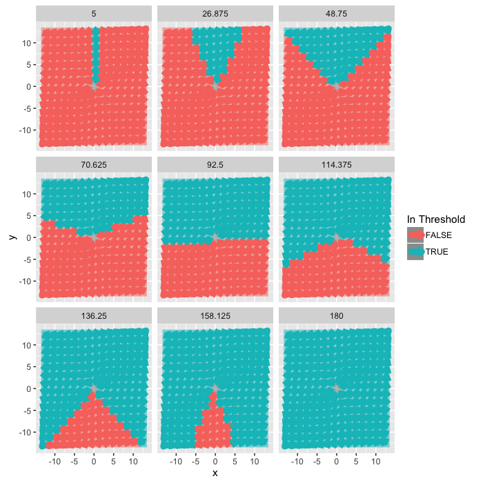
theme_bw(20)
A Machine Learning Approach to Image Processing
Segmentation and all the steps leading up to it are really a specialized type of learning problem.
lout<-21
b.grid<-expand.grid(x=seq(-10,10,length.out=lout),y=seq(-10,10,length.out=lout))
ring.image<-mutate(
b.grid,
Intensity = abs(cos(sqrt(x^2+y^2)/15*6.28))
)
ring.image.dist<-ddply(ring.image,.(x,y),function(in.pts) {
in.pts$Distance<-with(in.pts,sqrt(
min(
x^2+y^2
)
))
in.pts
})
ring.image.seg<-mutate(ring.image.dist,
Segmented = ifelse(
Intensity>0.5 & Distance>5 & Distance<10,
"Foreground","Background")
)
ring.image.seg<-mutate(ring.image.seg,
x=round(x+11),
y=round(y+11))
ring.im<-df.to.im(mutate(
b.grid,
val = 127*(abs(cos(sqrt(x^2+y^2)/15*6.28))+runif(nrow(b.grid)))
))
ring.img<-im.to.df(ring.im,out.col="Intensity")
blur.img<-im.to.df(gblur(ring.im,0.5),out.col="Intensity")
med.img<-im.to.df(medianFilter(ring.im/255,3)*255.0,out.col="Intensity")
Returning to the ring image we had before, we start with our knowledge or ground-truth of the ring
ggplot(ring.image.seg,aes(x,y,fill=Segmented))+
geom_raster()+
coord_equal()+
theme_bw(15)

Which we want to identify the from the following image by using image processing tools
simple.image<-ggplot(ring.img,aes(x,y,fill=Intensity))+
geom_tile()+
coord_equal()+
theme_bw(15)
simple.image

What does identify mean?
- Classify the pixels in the ring as Foreground
- Classify the pixels outside of the ring as Background
How do we quantify this?
- True Positive values in the ring that are classified as Foreground
- True Negative values outside the ring that are classified as Background
- False Positive values outside the ring that are classified as Foreground
- False Negative values in the ring that are classified as Background
tr.seg.img<-
mutate(ring.img,Segmented=ifelse(Intensity>170,"Foreground","Background"))[,
c("x","y","Segmented")]
gr.truth.img<-ring.image.seg[,c("x","y","Segmented")]
ggplot(tr.seg.img,
aes(x,y,fill=Segmented))+
geom_tile(color="black")+
coord_equal()+
labs(fill="Threshold\nSegmentation")+
theme_bw(15)

We can then apply a threshold to the image to determine the number of points in each category
score.img<-mutate(
merge(tr.seg.img,gr.truth.img,by=c("x","y"),suffixes=c("C","GT")),
Match=(SegmentedC==SegmentedGT),
Category=
ifelse(Match,
ifelse(SegmentedC=="Foreground","True Positive","True Negative"),
ifelse(SegmentedC=="Foreground","False Positive","False Negative")
)
)
ggplot(score.img,
aes(x,y,fill=SegmentedC,color=SegmentedGT))+
geom_tile(size=1)+
facet_wrap(~Category)+
coord_equal()+
scale_colour_manual(values=c("green","black"))+
scale_fill_manual(values=c("red","blue"))+
labs(fill="Threshold\nSegmentation",color="Ground\nTruth")+
theme_bw(20)

Ring Threshold Example
Try a number of different threshold values on the image and compare them to the original classification
mk.th.img<-function(in.img,steps,smin=0.3,smax=0.7) ldply(seq(smin,smax,length.out=steps),function(c.thresh) {
mutate(in.img,
Segmented = ifelse(
Intensity>c.thresh*255,
"Foreground","Background"),
Thresh = c.thresh
)
})
ggplot(mk.th.img(ring.img,9),aes(x,y,fill=Segmented))+
geom_tile(color="black")+
coord_equal()+
facet_wrap(~Thresh)+
theme_bw(15)

mk.stat.table<-function(in.img,steps,smin=0.3,smax=0.7)
ddply(mk.th.img(in.img,steps,smin,smax),.(Thresh),function(c.img) {
in.df<-merge(c.img[,c("x","y","Segmented")],
ring.image.seg[,c("x","y","Segmented")],
by=c("x","y"),suffixes=c("C","GT"))
in.df<-mutate(in.df,Match=(SegmentedC==SegmentedGT))
data.frame(TP=nrow(subset(in.df,SegmentedGT=="Foreground" & Match)),
TN=nrow(subset(in.df,SegmentedGT=="Background" & Match)),
FP=nrow(subset(in.df,SegmentedC=="Foreground" & !Match)),
FN=nrow(subset(in.df,SegmentedC=="Background" & !Match))
)
})
tp.table<-mk.stat.table(ring.img,6,smin=0,smax=1)
kable(tp.table)
Thresh
TP
TN
FP
FN
0.0
224
0
217
0
0.2
224
25
192
0
0.4
215
83
134
9
0.6
138
170
47
86
0.8
55
212
5
169
1.0
0
217
0
224
ggplot(melt(tp.table,id.vars=c("Thresh")),
aes(x=Thresh*100,y=100*value/200,color=variable))+
geom_point()+
geom_path()+
labs(color="",y="Percent (%)",x="Threshold Value (%)")+
theme_bw(20)

Apply Precision and Recall
- Recall (sensitivity)= TP/(TP + FN)
- Precision = TP/(TP + FP)
prec.table<-mutate(mk.stat.table(ring.img,6),
Recall=round(100*TP/(TP+FN)),
Precision=round(100*TP/(TP+FP))
)
kable(prec.table)
Thresh
TP
TN
FP
FN
Recall
Precision
0.30
221
51
166
3
99
57
0.38
218
76
141
6
97
61
0.46
204
106
111
20
91
65
0.54
164
146
71
60
73
70
0.62
128
178
39
96
57
77
0.70
100
200
17
124
45
85
ROC Curve
Reciever Operating Characteristic (first developed for WW2 soldiers detecting objects in battlefields using radar). The ideal is the top-right (identify everything and miss nothing)
prec.table<-mutate(mk.stat.table(ring.img,100),
Recall=TP/(TP+FN),
Precision=TP/(TP+FP)
)
ggplot(prec.table,aes(x=Recall,y=Precision))+
geom_point(aes(color=Thresh,shape="Image"),size=5)+
geom_point(data=data.frame(Recall=1,Precision=1),
aes(shape="Ideal"),size=5,color="red")+
geom_path()+
#coord_equal()+
scale_color_gradientn(colours=rainbow(6))+
labs(shape="")+
theme_bw(20)

Comparing Different Filters
We can then use this ROC curve to compare different filters (or even entire workflows), if the area is higher the approach is better.
all.img<-rbind(
cbind(mk.th.img(ring.img,3), name="Normal"),
cbind(mk.th.img(blur.img,3), name="Gaussian"),
cbind(mk.th.img(med.img,3), name="Median")
)
simple.image<-ggplot(all.img,aes(x,y,fill=Segmented))+
geom_tile(color="black")+
coord_equal()+
facet_grid(name~Thresh)+
theme_bw(15)
simple.image

Different approaches can be compared by area under the curve
stab<-function(img) mk.stat.table(img,100,smin=0.05,smax=0.95)
all.table<-rbind(
cbind(stab(ring.img), name="Normal"),
cbind(stab(blur.img), name="Gaussian"),
cbind(stab(med.img), name="Median")
)
prec.table<-mutate(all.table,
Recall=TP/(TP+FN),
Precision=TP/(TP+FP)
)
ggplot(prec.table,aes(x=Recall,y=Precision,color=name))+
geom_point(aes(shape="Image"),size=5)+
geom_point(data=data.frame(Recall=1,Precision=1),
aes(shape="Ideal"),size=5,color="red")+
geom_path()+
#coord_equal()+
labs(shape="",color="Filter")+
xlim(0.5,1)+ylim(0.5,1)+
theme_bw(20)

True Positive Rate and False Positive Rate
Another way of showing the ROC curve (more common for machine learning rather than medical diagnosis) is using the True positive rate and False positive rate
- True Positive Rate (recall)= TP/(TP + FN)
- False Positive Rate = FP/(FP + TN)
These show very similar information with the major difference being the goal is to be in the upper left-hand corner. Additionally random guesses can be shown as the slope 1 line. Therefore for a system to be useful it must lie above the random line.
tp.table<-mutate(all.table,
TPRate=TP/(TP+FN),
FPRate=FP/(FP+TN)
)
ggplot(tp.table,aes(x=FPRate,y=TPRate,color=name))+
geom_point(aes(shape="Image"),size=2)+
geom_point(data=data.frame(TPRate=1,FPRate=0),
aes(shape="Ideal"),size=5,color="red")+
geom_path()+
geom_segment(x=0,xend=1,y=0,yend=1,aes(color="Random Guess"))+
xlim(0,1)+ylim(0,1)+coord_equal()+
labs(shape="",x="False Positive Rate",y="True Positive Rate",linetype="")+
theme_bw(20)

Evaluating Models
- https://github.com/jvns/talks/blob/master/pydatanyc2014/slides.md
- http://mathbabe.org/2012/03/06/the-value-added-teacher-model-sucks/
Practical Example: Self-Driving Cars, Finding the Road
A more complicated example is finding the road in an image with cars and buildings
# image data
road.rgb.arr<-readJPEG(qbi.data("road_image.jpg"))
road.arr<-((road.rgb.arr[,,1]+road.rgb.arr[,,2]+road.rgb.arr[,,3])/3) %>% t %>% flip
## Error in asub.default(x, seq.int(dim(x)[2], 1), 2): could not find function "Quote"
road.image<- road.arr %>% im.to.df
## Error in eval(expr, envir, enclos): object 'road.arr' not found
# ground truth
cal.image<-readJPEG(qbi.data("road_image_street_bw.jpg")) %>% t %>% flip %>% im.to.df %>%
mutate(Segmented = ifelse(val,"Road","Background"))
## Error in asub.default(x, seq.int(dim(x)[2], 1), 2): could not find function "Quote"

ggplot(road.image,
aes(x,y,fill=val))+
geom_raster()+
coord_equal()+
scale_fill_gradientn(colours=c("black","white"))+
guides(fill=F)+
theme_bw(20)
From these images, an expert labeled the calcifications by hand, so we have ground truth data on where they are:
ggplot(cal.image,aes(x,y,fill=Segmented,alpha=Segmented))+
geom_raster()+
coord_equal()+
guides(alpha=F)+
theme_bw(20)
## Error in ggplot(cal.image, aes(x, y, fill = Segmented, alpha = Segmented)): object 'cal.image' not found
Applying a threshold
We can perform the same analysis on an image like this one, again using a simple threshold to evalulate how accurately we identify the stripes. Since they are white, we can selectively keep the white components.
tr.road<-mutate(road.image,
Segmented=ifelse(val>0.75,"Road","Background")
)
## Error in mutate_(.data, .dots = lazyeval::lazy_dots(...)): object 'road.image' not found
ggplot(tr.road,aes(x,y,fill=Segmented,alpha=val))+
geom_raster()+
coord_equal()+
guides(alpha=F)+
theme_bw(20)
## Error in ggplot(tr.road, aes(x, y, fill = Segmented, alpha = val)): object 'tr.road' not found
score.img<-mutate(
merge(tr.road[,c("x","y","Segmented")],
cal.image[,c("x","y","Segmented")],
by=c("x","y"),suffixes=c("C","GT")),
Match=(SegmentedC==SegmentedGT),
Category=
ifelse(Match,
ifelse(SegmentedC=="Road","True Positive","True Negative"),
ifelse(SegmentedC=="Road","False Positive","False Negative")
)
)
## Error in merge(tr.road[, c("x", "y", "Segmented")], cal.image[, c("x", : object 'tr.road' not found
ggplot(score.img,
aes(x,y,fill=SegmentedGT))+
geom_tile()+
facet_grid(Category~.)+
coord_equal()+
scale_colour_manual(values=c("green","black"))+
scale_fill_manual(values=c("red","blue"))+
labs(fill="Ground\nTruth")+
theme_bw(20)

Examining the ROC Curve
mk.th.img<-function(in.img,stepseq) ldply(stepseq,function(c.thresh) {
mutate(in.img,
Segmented = ifelse(
val>c.thresh,
"Road","Background"),
Thresh = c.thresh
)
})
mk.stat.table<-function(in.img,stepseq)
ddply(mk.th.img(in.img,stepseq),.(Thresh),function(c.img) {
in.df<-merge(c.img[,c("x","y","Segmented")],
cal.image[,c("x","y","Segmented")],
by=c("x","y"),suffixes=c("C","GT"))
in.df<-mutate(in.df,Match=(SegmentedC==SegmentedGT))
data.frame(TP=nrow(subset(in.df,SegmentedGT=="Road" & Match)),
TN=nrow(subset(in.df,SegmentedGT=="Background" & Match)),
FP=nrow(subset(in.df,SegmentedC=="Road" & !Match)),
FN=nrow(subset(in.df,SegmentedC=="Background" & !Match))
)
})
step.fcn<-function(vals,n) quantile(vals,seq(0,1,length.out=n+2)[-c(1,n+2)])
abs.steps<-step.fcn(road.image$val,6)
## Error in quantile(vals, seq(0, 1, length.out = n + 2)[-c(1, n + 2)]): object 'road.image' not found
tp.table<-mk.stat.table(road.image,abs.steps)
## Error in inherits(.data, "split"): object 'abs.steps' not found
prec.table<-mutate(tp.table,
Thresh=round(100*Thresh),
Recall=round(100*TP/(TP+FN)),
Precision=round(100*TP/(TP+FP))
)
kable(prec.table)
Thresh
TP
TN
FP
FN
name
TPRate
FPRate
Recall
Precision
5
224
0
217
0
Normal
1.0000000
1.0000000
100
51
6
224
0
217
0
Normal
1.0000000
1.0000000
100
51
7
224
1
216
0
Normal
1.0000000
0.9953917
100
51
8
224
1
216
0
Normal
1.0000000
0.9953917
100
51
9
224
1
216
0
Normal
1.0000000
0.9953917
100
51
10
224
2
215
0
Normal
1.0000000
0.9907834
100
51
10
224
3
214
0
Normal
1.0000000
0.9861751
100
51
11
224
7
210
0
Normal
1.0000000
0.9677419
100
52
12
224
8
209
0
Normal
1.0000000
0.9631336
100
52
13
224
8
209
0
Normal
1.0000000
0.9631336
100
52
14
224
8
209
0
Normal
1.0000000
0.9631336
100
52
15
224
11
206
0
Normal
1.0000000
0.9493088
100
52
16
224
16
201
0
Normal
1.0000000
0.9262673
100
53
17
224
17
200
0
Normal
1.0000000
0.9216590
100
53
18
224
20
197
0
Normal
1.0000000
0.9078341
100
53
19
224
21
196
0
Normal
1.0000000
0.9032258
100
53
20
224
24
193
0
Normal
1.0000000
0.8894009
100
54
20
224
26
191
0
Normal
1.0000000
0.8801843
100
54
21
224
28
189
0
Normal
1.0000000
0.8709677
100
54
22
224
32
185
0
Normal
1.0000000
0.8525346
100
55
23
224
34
183
0
Normal
1.0000000
0.8433180
100
55
24
224
34
183
0
Normal
1.0000000
0.8433180
100
55
25
224
35
182
0
Normal
1.0000000
0.8387097
100
55
26
224
38
179
0
Normal
1.0000000
0.8248848
100
56
27
224
41
176
0
Normal
1.0000000
0.8110599
100
56
28
224
44
173
0
Normal
1.0000000
0.7972350
100
56
29
223
48
169
1
Normal
0.9955357
0.7788018
100
57
30
221
50
167
3
Normal
0.9866071
0.7695853
99
57
30
221
51
166
3
Normal
0.9866071
0.7649770
99
57
31
221
55
162
3
Normal
0.9866071
0.7465438
99
58
32
221
59
158
3
Normal
0.9866071
0.7281106
99
58
33
221
66
151
3
Normal
0.9866071
0.6958525
99
59
34
221
68
149
3
Normal
0.9866071
0.6866359
99
60
35
220
70
147
4
Normal
0.9821429
0.6774194
98
60
36
220
72
145
4
Normal
0.9821429
0.6682028
98
60
37
220
73
144
4
Normal
0.9821429
0.6635945
98
60
38
219
76
141
5
Normal
0.9776786
0.6497696
98
61
39
217
77
140
7
Normal
0.9687500
0.6451613
97
61
40
216
81
136
8
Normal
0.9642857
0.6267281
96
61
40
214
85
132
10
Normal
0.9553571
0.6082949
96
62
41
213
87
130
11
Normal
0.9508929
0.5990783
95
62
42
212
89
128
12
Normal
0.9464286
0.5898618
95
62
43
208
95
122
16
Normal
0.9285714
0.5622120
93
63
44
207
100
117
17
Normal
0.9241071
0.5391705
92
64
45
205
103
114
19
Normal
0.9151786
0.5253456
92
64
46
204
106
111
20
Normal
0.9107143
0.5115207
91
65
47
201
112
105
23
Normal
0.8973214
0.4838710
90
66
48
200
115
102
24
Normal
0.8928571
0.4700461
89
66
49
198
118
99
26
Normal
0.8839286
0.4562212
88
67
50
192
124
93
32
Normal
0.8571429
0.4285714
86
67
50
188
130
87
36
Normal
0.8392857
0.4009217
84
68
51
180
131
86
44
Normal
0.8035714
0.3963134
80
68
52
172
134
83
52
Normal
0.7678571
0.3824885
77
67
53
168
141
76
56
Normal
0.7500000
0.3502304
75
69
54
164
146
71
60
Normal
0.7321429
0.3271889
73
70
55
160
149
68
64
Normal
0.7142857
0.3133641
71
70
56
157
149
68
67
Normal
0.7008929
0.3133641
70
70
57
152
157
60
72
Normal
0.6785714
0.2764977
68
72
58
150
161
56
74
Normal
0.6696429
0.2580645
67
73
59
144
165
52
80
Normal
0.6428571
0.2396313
64
73
60
138
170
47
86
Normal
0.6160714
0.2165899
62
75
60
135
175
42
89
Normal
0.6026786
0.1935484
60
76
61
129
176
41
95
Normal
0.5758929
0.1889401
58
76
62
128
178
39
96
Normal
0.5714286
0.1797235
57
77
63
127
180
37
97
Normal
0.5669643
0.1705069
57
77
64
124
182
35
100
Normal
0.5535714
0.1612903
55
78
65
120
185
32
104
Normal
0.5357143
0.1474654
54
79
66
119
189
28
105
Normal
0.5312500
0.1290323
53
81
67
114
194
23
110
Normal
0.5089286
0.1059908
51
83
68
108
196
21
116
Normal
0.4821429
0.0967742
48
84
69
106
198
19
118
Normal
0.4732143
0.0875576
47
85
70
101
200
17
123
Normal
0.4508929
0.0783410
45
86
70
96
200
17
128
Normal
0.4285714
0.0783410
43
85
71
85
202
15
139
Normal
0.3794643
0.0691244
38
85
72
82
204
13
142
Normal
0.3660714
0.0599078
37
86
73
80
207
10
144
Normal
0.3571429
0.0460829
36
89
74
80
208
9
144
Normal
0.3571429
0.0414747
36
90
75
78
211
6
146
Normal
0.3482143
0.0276498
35
93
76
76
212
5
148
Normal
0.3392857
0.0230415
34
94
77
71
212
5
153
Normal
0.3169643
0.0230415
32
93
78
70
212
5
154
Normal
0.3125000
0.0230415
31
93
79
65
212
5
159
Normal
0.2901786
0.0230415
29
93
80
59
212
5
165
Normal
0.2633929
0.0230415
26
92
80
55
212
5
169
Normal
0.2455357
0.0230415
25
92
81
50
212
5
174
Normal
0.2232143
0.0230415
22
91
82
44
214
3
180
Normal
0.1964286
0.0138249
20
94
83
42
215
2
182
Normal
0.1875000
0.0092166
19
95
84
41
215
2
183
Normal
0.1830357
0.0092166
18
95
85
39
215
2
185
Normal
0.1741071
0.0092166
17
95
86
32
217
0
192
Normal
0.1428571
0.0000000
14
100
87
28
217
0
196
Normal
0.1250000
0.0000000
12
100
88
27
217
0
197
Normal
0.1205357
0.0000000
12
100
89
25
217
0
199
Normal
0.1116071
0.0000000
11
100
90
23
217
0
201
Normal
0.1026786
0.0000000
10
100
90
22
217
0
202
Normal
0.0982143
0.0000000
10
100
91
20
217
0
204
Normal
0.0892857
0.0000000
9
100
92
17
217
0
207
Normal
0.0758929
0.0000000
8
100
93
16
217
0
208
Normal
0.0714286
0.0000000
7
100
94
10
217
0
214
Normal
0.0446429
0.0000000
4
100
95
7
217
0
217
Normal
0.0312500
0.0000000
3
100
5
224
0
217
0
Gaussian
1.0000000
1.0000000
100
51
6
224
0
217
0
Gaussian
1.0000000
1.0000000
100
51
7
224
0
217
0
Gaussian
1.0000000
1.0000000
100
51
8
224
0
217
0
Gaussian
1.0000000
1.0000000
100
51
9
224
0
217
0
Gaussian
1.0000000
1.0000000
100
51
10
224
0
217
0
Gaussian
1.0000000
1.0000000
100
51
10
224
0
217
0
Gaussian
1.0000000
1.0000000
100
51
11
224
0
217
0
Gaussian
1.0000000
1.0000000
100
51
12
224
0
217
0
Gaussian
1.0000000
1.0000000
100
51
13
224
0
217
0
Gaussian
1.0000000
1.0000000
100
51
14
224
0
217
0
Gaussian
1.0000000
1.0000000
100
51
15
224
0
217
0
Gaussian
1.0000000
1.0000000
100
51
16
224
1
216
0
Gaussian
1.0000000
0.9953917
100
51
17
224
1
216
0
Gaussian
1.0000000
0.9953917
100
51
18
224
1
216
0
Gaussian
1.0000000
0.9953917
100
51
19
224
1
216
0
Gaussian
1.0000000
0.9953917
100
51
20
224
2
215
0
Gaussian
1.0000000
0.9907834
100
51
20
224
3
214
0
Gaussian
1.0000000
0.9861751
100
51
21
224
3
214
0
Gaussian
1.0000000
0.9861751
100
51
22
224
5
212
0
Gaussian
1.0000000
0.9769585
100
51
23
224
8
209
0
Gaussian
1.0000000
0.9631336
100
52
24
224
9
208
0
Gaussian
1.0000000
0.9585253
100
52
25
224
12
205
0
Gaussian
1.0000000
0.9447005
100
52
26
224
14
203
0
Gaussian
1.0000000
0.9354839
100
52
27
224
18
199
0
Gaussian
1.0000000
0.9170507
100
53
28
224
20
197
0
Gaussian
1.0000000
0.9078341
100
53
29
224
22
195
0
Gaussian
1.0000000
0.8986175
100
53
30
224
26
191
0
Gaussian
1.0000000
0.8801843
100
54
30
224
30
187
0
Gaussian
1.0000000
0.8617512
100
55
31
224
36
181
0
Gaussian
1.0000000
0.8341014
100
55
32
224
39
178
0
Gaussian
1.0000000
0.8202765
100
56
33
224
43
174
0
Gaussian
1.0000000
0.8018433
100
56
34
223
47
170
1
Gaussian
0.9955357
0.7834101
100
57
35
223
54
163
1
Gaussian
0.9955357
0.7511521
100
58
36
223
58
159
1
Gaussian
0.9955357
0.7327189
100
58
37
223
61
156
1
Gaussian
0.9955357
0.7188940
100
59
38
222
66
151
2
Gaussian
0.9910714
0.6958525
99
60
39
221
68
149
3
Gaussian
0.9866071
0.6866359
99
60
40
221
74
143
3
Gaussian
0.9866071
0.6589862
99
61
40
220
77
140
4
Gaussian
0.9821429
0.6451613
98
61
41
219
82
135
5
Gaussian
0.9776786
0.6221198
98
62
42
219
88
129
5
Gaussian
0.9776786
0.5944700
98
63
43
218
94
123
6
Gaussian
0.9732143
0.5668203
97
64
44
217
99
118
7
Gaussian
0.9687500
0.5437788
97
65
45
217
100
117
7
Gaussian
0.9687500
0.5391705
97
65
46
216
106
111
8
Gaussian
0.9642857
0.5115207
96
66
47
214
110
107
10
Gaussian
0.9553571
0.4930876
96
67
48
213
115
102
11
Gaussian
0.9508929
0.4700461
95
68
49
209
125
92
15
Gaussian
0.9330357
0.4239631
93
69
50
208
133
84
16
Gaussian
0.9285714
0.3870968
93
71
50
207
139
78
17
Gaussian
0.9241071
0.3594470
92
73
51
205
142
75
19
Gaussian
0.9151786
0.3456221
92
73
52
202
149
68
22
Gaussian
0.9017857
0.3133641
90
75
53
194
154
63
30
Gaussian
0.8660714
0.2903226
87
75
54
189
162
55
35
Gaussian
0.8437500
0.2534562
84
77
55
181
167
50
43
Gaussian
0.8080357
0.2304147
81
78
56
178
171
46
46
Gaussian
0.7946429
0.2119816
79
79
57
170
174
43
54
Gaussian
0.7589286
0.1981567
76
80
58
164
177
40
60
Gaussian
0.7321429
0.1843318
73
80
59
159
180
37
65
Gaussian
0.7098214
0.1705069
71
81
60
151
185
32
73
Gaussian
0.6741071
0.1474654
67
83
60
148
189
28
76
Gaussian
0.6607143
0.1290323
66
84
61
144
191
26
80
Gaussian
0.6428571
0.1198157
64
85
62
138
196
21
86
Gaussian
0.6160714
0.0967742
62
87
63
130
198
19
94
Gaussian
0.5803571
0.0875576
58
87
64
127
200
17
97
Gaussian
0.5669643
0.0783410
57
88
65
121
202
15
103
Gaussian
0.5401786
0.0691244
54
89
66
112
203
14
112
Gaussian
0.5000000
0.0645161
50
89
67
109
204
13
115
Gaussian
0.4866071
0.0599078
49
89
68
102
206
11
122
Gaussian
0.4553571
0.0506912
46
90
69
100
210
7
124
Gaussian
0.4464286
0.0322581
45
93
70
93
211
6
131
Gaussian
0.4151786
0.0276498
42
94
70
82
212
5
142
Gaussian
0.3660714
0.0230415
37
94
71
77
213
4
147
Gaussian
0.3437500
0.0184332
34
95
72
72
213
4
152
Gaussian
0.3214286
0.0184332
32
95
73
70
213
4
154
Gaussian
0.3125000
0.0184332
31
95
74
64
213
4
160
Gaussian
0.2857143
0.0184332
29
94
75
58
213
4
166
Gaussian
0.2589286
0.0184332
26
94
76
55
215
2
169
Gaussian
0.2455357
0.0092166
25
96
77
47
215
2
177
Gaussian
0.2098214
0.0092166
21
96
78
44
215
2
180
Gaussian
0.1964286
0.0092166
20
96
79
38
217
0
186
Gaussian
0.1696429
0.0000000
17
100
80
33
217
0
191
Gaussian
0.1473214
0.0000000
15
100
80
30
217
0
194
Gaussian
0.1339286
0.0000000
13
100
81
25
217
0
199
Gaussian
0.1116071
0.0000000
11
100
82
22
217
0
202
Gaussian
0.0982143
0.0000000
10
100
83
18
217
0
206
Gaussian
0.0803571
0.0000000
8
100
84
15
217
0
209
Gaussian
0.0669643
0.0000000
7
100
85
11
217
0
213
Gaussian
0.0491071
0.0000000
5
100
86
10
217
0
214
Gaussian
0.0446429
0.0000000
4
100
87
7
217
0
217
Gaussian
0.0312500
0.0000000
3
100
88
5
217
0
219
Gaussian
0.0223214
0.0000000
2
100
89
3
217
0
221
Gaussian
0.0133929
0.0000000
1
100
90
1
217
0
223
Gaussian
0.0044643
0.0000000
0
100
90
1
217
0
223
Gaussian
0.0044643
0.0000000
0
100
91
0
217
0
224
Gaussian
0.0000000
0.0000000
0
NaN
92
0
217
0
224
Gaussian
0.0000000
0.0000000
0
NaN
93
0
217
0
224
Gaussian
0.0000000
0.0000000
0
NaN
94
0
217
0
224
Gaussian
0.0000000
0.0000000
0
NaN
95
0
217
0
224
Gaussian
0.0000000
0.0000000
0
NaN
5
224
0
217
0
Median
1.0000000
1.0000000
100
51
6
224
0
217
0
Median
1.0000000
1.0000000
100
51
7
224
0
217
0
Median
1.0000000
1.0000000
100
51
8
224
0
217
0
Median
1.0000000
1.0000000
100
51
9
224
0
217
0
Median
1.0000000
1.0000000
100
51
10
224
0
217
0
Median
1.0000000
1.0000000
100
51
10
224
0
217
0
Median
1.0000000
1.0000000
100
51
11
224
0
217
0
Median
1.0000000
1.0000000
100
51
12
224
0
217
0
Median
1.0000000
1.0000000
100
51
13
224
0
217
0
Median
1.0000000
1.0000000
100
51
14
224
0
217
0
Median
1.0000000
1.0000000
100
51
15
224
0
217
0
Median
1.0000000
1.0000000
100
51
16
224
0
217
0
Median
1.0000000
1.0000000
100
51
17
224
0
217
0
Median
1.0000000
1.0000000
100
51
18
224
0
217
0
Median
1.0000000
1.0000000
100
51
19
224
0
217
0
Median
1.0000000
1.0000000
100
51
20
224
0
217
0
Median
1.0000000
1.0000000
100
51
20
224
0
217
0
Median
1.0000000
1.0000000
100
51
21
224
0
217
0
Median
1.0000000
1.0000000
100
51
22
224
0
217
0
Median
1.0000000
1.0000000
100
51
23
224
0
217
0
Median
1.0000000
1.0000000
100
51
24
224
0
217
0
Median
1.0000000
1.0000000
100
51
25
224
0
217
0
Median
1.0000000
1.0000000
100
51
26
224
0
217
0
Median
1.0000000
1.0000000
100
51
27
224
0
217
0
Median
1.0000000
1.0000000
100
51
28
224
0
217
0
Median
1.0000000
1.0000000
100
51
29
224
0
217
0
Median
1.0000000
1.0000000
100
51
30
224
0
217
0
Median
1.0000000
1.0000000
100
51
30
224
0
217
0
Median
1.0000000
1.0000000
100
51
31
224
0
217
0
Median
1.0000000
1.0000000
100
51
32
224
0
217
0
Median
1.0000000
1.0000000
100
51
33
224
1
216
0
Median
1.0000000
0.9953917
100
51
34
224
1
216
0
Median
1.0000000
0.9953917
100
51
35
224
1
216
0
Median
1.0000000
0.9953917
100
51
36
224
2
215
0
Median
1.0000000
0.9907834
100
51
37
224
2
215
0
Median
1.0000000
0.9907834
100
51
38
224
2
215
0
Median
1.0000000
0.9907834
100
51
39
224
2
215
0
Median
1.0000000
0.9907834
100
51
40
224
2
215
0
Median
1.0000000
0.9907834
100
51
40
224
2
215
0
Median
1.0000000
0.9907834
100
51
41
224
2
215
0
Median
1.0000000
0.9907834
100
51
42
224
3
214
0
Median
1.0000000
0.9861751
100
51
43
224
4
213
0
Median
1.0000000
0.9815668
100
51
44
224
5
212
0
Median
1.0000000
0.9769585
100
51
45
223
7
210
1
Median
0.9955357
0.9677419
100
52
46
222
11
206
2
Median
0.9910714
0.9493088
99
52
47
222
17
200
2
Median
0.9910714
0.9216590
99
53
48
222
20
197
2
Median
0.9910714
0.9078341
99
53
49
222
21
196
2
Median
0.9910714
0.9032258
99
53
50
222
39
178
2
Median
0.9910714
0.8202765
99
56
50
222
60
157
2
Median
0.9910714
0.7235023
99
59
51
220
69
148
4
Median
0.9821429
0.6820276
98
60
52
218
85
132
6
Median
0.9732143
0.6082949
97
62
53
214
119
98
10
Median
0.9553571
0.4516129
96
69
54
200
142
75
24
Median
0.8928571
0.3456221
89
73
55
188
155
62
36
Median
0.8392857
0.2857143
84
75
56
179
157
60
45
Median
0.7991071
0.2764977
80
75
57
144
175
42
80
Median
0.6428571
0.1935484
64
77
58
121
182
35
103
Median
0.5401786
0.1612903
54
78
59
82
191
26
142
Median
0.3660714
0.1198157
37
76
60
65
204
13
159
Median
0.2901786
0.0599078
29
83
60
52
206
11
172
Median
0.2321429
0.0506912
23
83
61
39
209
8
185
Median
0.1741071
0.0368664
17
83
62
37
209
8
187
Median
0.1651786
0.0368664
17
82
63
34
210
7
190
Median
0.1517857
0.0322581
15
83
64
24
210
7
200
Median
0.1071429
0.0322581
11
77
65
14
213
4
210
Median
0.0625000
0.0184332
6
78
66
9
214
3
215
Median
0.0401786
0.0138249
4
75
67
5
216
1
219
Median
0.0223214
0.0046083
2
83
68
0
217
0
224
Median
0.0000000
0.0000000
0
NaN
69
0
217
0
224
Median
0.0000000
0.0000000
0
NaN
70
0
217
0
224
Median
0.0000000
0.0000000
0
NaN
70
0
217
0
224
Median
0.0000000
0.0000000
0
NaN
71
0
217
0
224
Median
0.0000000
0.0000000
0
NaN
72
0
217
0
224
Median
0.0000000
0.0000000
0
NaN
73
0
217
0
224
Median
0.0000000
0.0000000
0
NaN
74
0
217
0
224
Median
0.0000000
0.0000000
0
NaN
75
0
217
0
224
Median
0.0000000
0.0000000
0
NaN
76
0
217
0
224
Median
0.0000000
0.0000000
0
NaN
77
0
217
0
224
Median
0.0000000
0.0000000
0
NaN
78
0
217
0
224
Median
0.0000000
0.0000000
0
NaN
79
0
217
0
224
Median
0.0000000
0.0000000
0
NaN
80
0
217
0
224
Median
0.0000000
0.0000000
0
NaN
80
0
217
0
224
Median
0.0000000
0.0000000
0
NaN
81
0
217
0
224
Median
0.0000000
0.0000000
0
NaN
82
0
217
0
224
Median
0.0000000
0.0000000
0
NaN
83
0
217
0
224
Median
0.0000000
0.0000000
0
NaN
84
0
217
0
224
Median
0.0000000
0.0000000
0
NaN
85
0
217
0
224
Median
0.0000000
0.0000000
0
NaN
86
0
217
0
224
Median
0.0000000
0.0000000
0
NaN
87
0
217
0
224
Median
0.0000000
0.0000000
0
NaN
88
0
217
0
224
Median
0.0000000
0.0000000
0
NaN
89
0
217
0
224
Median
0.0000000
0.0000000
0
NaN
90
0
217
0
224
Median
0.0000000
0.0000000
0
NaN
90
0
217
0
224
Median
0.0000000
0.0000000
0
NaN
91
0
217
0
224
Median
0.0000000
0.0000000
0
NaN
92
0
217
0
224
Median
0.0000000
0.0000000
0
NaN
93
0
217
0
224
Median
0.0000000
0.0000000
0
NaN
94
0
217
0
224
Median
0.0000000
0.0000000
0
NaN
95
0
217
0
224
Median
0.0000000
0.0000000
0
NaN
abs.steps<-step.fcn(road.image$val,15)
## Error in quantile(vals, seq(0, 1, length.out = n + 2)[-c(1, n + 2)]): object 'road.image' not found
tp.table<-mk.stat.table(road.image,abs.steps)
## Error in inherits(.data, "split"): object 'abs.steps' not found
ggplot(melt(tp.table,id.vars=c("Thresh")),
aes(x=Thresh*100,y=value,color=variable))+
geom_point()+
geom_path()+
labs(color="",y="Pixel Count",x="Threshold Value (%)")+
scale_y_sqrt()+
theme_bw(20)
## Error in self$trans$transform(x): non-numeric argument to mathematical function

prec.table<-mutate(tp.table,
Recall=TP/(TP+FN),
Precision=TP/(TP+FP)
)
ggplot(prec.table,aes(x=Recall,y=Precision))+
geom_point(aes(color=Thresh,shape="Image"),size=5)+
geom_point(data=data.frame(Recall=1,Precision=1),
aes(shape="Ideal"),size=5,color="red")+
geom_path()+
scale_color_gradientn(colours=rainbow(6))+
scale_x_sqrt()+
labs(shape="")+
theme_bw(20)

ROC: True Positive Rate vs False Positive
tpr.table<-mutate(tp.table,
TPRate=TP/(TP+FN),
FPRate=FP/(FP+TN)
)
ggplot(tpr.table,aes(x=FPRate,y=TPRate))+
geom_point(aes(shape="Image"),size=2)+
geom_point(data=data.frame(TPRate=1,FPRate=0),
aes(shape="Ideal"),size=5,color="red")+
geom_path()+
geom_segment(x=0,xend=1,y=0,yend=1,aes(color="Random Guess"))+
xlim(0,1)+ylim(0,1)+coord_equal()+
labs(shape="",x="False Positive Rate",y="True Positive Rate",linetype="")+
theme_bw(20)

Using other pieces of information
Since we know the stripes are on the road, we can add another criteria (just the lower half), we can improve the ROC curve substantially.
# subtract blur
#road.blur <- (road.arr - gblur(road.arr,2)) %>% im.to.df
roi.road.image<-road.image %>%
mutate(val =
ifelse(x>200,ifelse(y<200,val,0),0)
)
## Error in eval(expr, envir, enclos): object 'road.image' not found
dci.steps<-step.fcn(roi.road.image$val,12)
## Error in quantile(vals, seq(0, 1, length.out = n + 2)[-c(1, n + 2)]): object 'roi.road.image' not found
dci.table<-mk.stat.table(roi.road.image,dci.steps)
## Error in inherits(.data, "split"): object 'dci.steps' not found
prec.dci.table<-mutate(dci.table,
Recall=TP/(TP+FN),
Precision=TP/(TP+FP)
)
## Error in mutate_(.data, .dots = lazyeval::lazy_dots(...)): object 'dci.table' not found
ggplot(roi.road.image,
aes(x,y,fill=val))+
geom_tile()+
coord_equal()+
scale_fill_gradientn(colours=c("black","white"))+
guides(fill=F)+
theme_bw(20)
## Error in ggplot(roi.road.image, aes(x, y, fill = val)): object 'roi.road.image' not found
# subtract blur
# road.blur <- (road.arr - gblur(road.arr,2)) %>% im.to.df
roi.blur.image<-gblur(road.arr,2) %>% im.to.df %>%
mutate(val =
ifelse(x>200,ifelse(y<200,val,0),0)
)
## Error in validObject(x): object 'road.arr' not found
blur.steps<-step.fcn(roi.blur.image$val,12)
## Error in quantile(vals, seq(0, 1, length.out = n + 2)[-c(1, n + 2)]): object 'roi.blur.image' not found
blur.table<-mk.stat.table(roi.blur.image,blur.steps)
## Error in inherits(.data, "split"): object 'blur.steps' not found
prec.blur.table<-mutate(blur.table,
Recall=TP/(TP+FN),
Precision=TP/(TP+FP)
)
## Error in mutate_(.data, .dots = lazyeval::lazy_dots(...)): object 'blur.table' not found
ggplot(roi.blur.image,
aes(x,y,fill=val))+
geom_tile()+
coord_equal()+
scale_fill_gradientn(colours=c("black","white"))+
guides(fill=F)+
theme_bw(20)
## Error in ggplot(roi.blur.image, aes(x, y, fill = val)): object 'roi.blur.image' not found
The resulting ROC curves
ggplot(rbind(cbind(prec.table,Channel="Standard"),
cbind(prec.dci.table,Channel="Region"),
cbind(prec.blur.table,Channel="Region Blur")
),
aes(x=Recall,y=Precision))+
geom_point(aes(shape="Image"),size=5)+
geom_point(data=data.frame(Recall=1,Precision=1),
aes(shape="Ideal"),size=5,color="red")+
geom_path(aes(group=Channel,color=Channel))+
scale_y_sqrt()+
labs(shape="")+
theme_bw(20)
## Error in cbind(prec.dci.table, Channel = "Region"): object 'prec.dci.table' not found
Other Image Types
Going beyond vector the possibilities for images are limitless. The following shows a tensor plot with the tensor represented as an ellipse.
$$ I(x,y) = \hat{f}(x,y) $$
nx<-4
ny<-4
n.pi<-4
grad.im<-expand.grid(x=c(-nx:nx)/nx*n.pi*pi,
y=c(-ny:ny)/ny*n.pi*pi)
grad.im<-cbind(grad.im,
col=1.5*with(grad.im,abs(cos(x*y))/(abs(x*y)+(3*pi/nx)))+
0.5*runif(nrow(grad.im)),
a=with(grad.im,sqrt(2/(abs(x)+0.5))),
b=with(grad.im,0.5*sqrt(abs(x)+1)),
th=0.5*runif(nrow(grad.im)),
aiso=1,count=1)
create.ellipse.points<-function(x.off=0,y.off=0,a=1,b=NULL,th.off=0,th.max=2*pi,pts=36,...) {
if (is.null(b)) b<-a
th<-seq(0,th.max,length.out=pts)
data.frame(x=a*cos(th.off)*cos(th)+b*sin(th.off)*sin(th)+x.off,
y=-1*a*sin(th.off)*cos(th)+b*cos(th.off)*sin(th)+y.off,
id=as.factor(paste(x.off,y.off,a,b,th.off,pts,sep=":")),...)
}
deform.ellipse.draw<-function(c.box) {
create.ellipse.points(x.off=c.box$x[1],
y.off=c.box$y[1],
a=c.box$a[1],
b=c.box$b[1],
th.off=c.box$th[1],
col=c.box$col[1])
}
# normalize vector
tens.im<-ddply(grad.im,.(x,y),deform.ellipse.draw)
ggplot(tens.im,aes(x=x,y=y,group=as.factor(id),fill=col))+
geom_polygon(color="black")+coord_fixed(ratio=1)+scale_fill_gradient(low="black",high="white")+guides(fill=F)+
theme_bw(20)
Once the variable count is above 2, individual density functions and a series of cross plots are easier to interpret than some multidimensional density hypervolume.
ggplot(grad.im)+
geom_histogram(aes(x=a,fill="Width"),alpha=0.7)+
geom_histogram(aes(x=b,fill="Height"),alpha=0.7)+
geom_histogram(aes(x=th,fill="Orientation"),alpha=0.7)+
geom_histogram(aes(x=col,fill="Color"),alpha=0.7)+
guides(color=F)+labs(fill="Variable")+
theme_bw(15)

plot(grad.im[,c("a","b","th","col")])

Multiple Phases: Segmenting Shale
% Shale provided from Kanitpanyacharoen, W. (2012). Synchrotron X-ray Applications Toward an Understanding of Elastic Anisotropy.
- Here we have a shale sample measured with X-ray tomography with three different phases inside (clay, rock, and air).
- The model is that because the chemical composition and density of each phase is different they will absorb different amounts of x-rays and appear as different brightnesses in the image
shaleImage<-im.to.df(jpeg::readJPEG("ext-figures/ShaleSample.jpg"))
ggplot(shaleImage,aes(x=x,y=y,fill=val))+
geom_tile()+
labs(fill="Absorption (au)")+theme_bw(20)

Ideally we would derive 3 values for the thresholds based on a model for the composition of each phase and how much it absorbs, but that is not always possible or practical.
- While there are 3 phases clearly visible in the image, the histogram is less telling (even after being re-scaled).

Multiple Segmentations
For this exercise we choose arbitrarily 3 ranges for the different phases and perform visual inspection

The relation can explicitly be written out as
$$ I(x) =
\begin{cases}
\text{Void}, & 0 \leq x \leq 0.2 \\
\text{Clay}, & 0.2 < x \leq 0.5 \\
\text{Rock}, & 0.5 < x
\end{cases}$$
ggplot(shale.vals,aes(x=x,y=y,fill=th.label,alpha=1-val))+coord_fixed(ratio=1)+
geom_raster()+guides(fill=F,alpha=F)+theme_bw(20)+facet_wrap(~th.label)

Implementation
The implementations of basic thresholds and segmentations is very easy since it is a unary operation of a single image
$$ f(I(\vec{x})) $$
In mathematical terms this is called a map and since it does not require information from neighboring voxels or images it can be calculated for each point independently (parallel). Filters on the other hand almost always depend on neighboring voxels and thus the calculations are not as easy to seperate.
Implementation Code
Matlab
The simplist is a single threshold in Matlab:
thresh_img = gray_img > thresh
A more complicated threshold:
thresh_img = (gray_img > thresh_a) & (gray_img > thresh_b)
Python (numpy)
thresh_img = gray_img > thresh
Python
thresh_img = map(lambda gray_val: gray_val>thresh,
gray_img)
Java
boolean[] thresh_img = new boolean[x_size*y_size*z_size];
for(int x=x_min;x<x_max;x++)
for(int y=y_min;y<y_max;y++)
for(int z=z_min;z<z_max;z++) {
int offset=(z*y_size+y)*x_size+x;
thresh_img[offset]=gray_img[offset]>thresh;
}
In C/C++
bool* thresh_img = malloc(x_size*y_size*z_size * sizeof (bool));
for(int x=x_min;x<x_max;x++)
for(int y=y_min;y<y_max;y++)
for(int z=z_min;z<z_max;z++) {
int offset=(z*y_size+y)*x_size+x;
thresh_img[offset]=gray_img[offset]>thresh;
}
Pitfalls with Segmentation
Partial Volume Effect
- The partial volume effect is the name for the effect of discretization on the image into pixels or voxels.
- Surfaces are complicated, voxels are simple boxes which make poor representations
- Many voxels are only partially filled, but only the voxels on the surface
- Removing the first layer alleviates issue
make.circle<-function(nx,r,nscale=1,
circ.fun=function(x,y,r) ((x^2+y^2)

binned.data<-
ddply.cutcols(subset(sph.list,val<0.25),.(cut_interval(val,20),r),function(x) data.frame(count=nrow(x)))
# mutate(binned.data,ncount=ifelse(count>10,10,count)),
aes(x=val)
- x -> val
ggplot(subset(sph.list,val<0.25),aes(y=as.factor(r),x=val))+
stat_bin2d(drop=T,bins=5)+
scale_fill_gradientn(colours=rainbow(5),trans="sqrt",lim=c(0,25),na.value="purple")+
theme_bw(20)+labs(x="Intensity",fill="Frequency",y="Radius")

Shown as a function of radius
pve.table<-ddply(sph.list,.(r),function(c.rad.df) data.frame(m.int=mean(c.rad.df$val),
m.sd=sd(c.rad.df$val)
)
)
names(pve.table)<-c("Radius","Mean Intensity","Sd Intensity")
kable(pve.table)
Radius
Mean Intensity
Sd Intensity
2.0
0.0311250
0.1623387
3.5
0.0960250
0.2770132
5.0
0.1956250
0.3825768
6.5
0.3311250
0.4510394
8.0
0.5017250
0.4819382
9.5
0.7072841
0.4258651
Morphology
Returning to the original image of a cross
nx<-8
ny<-8
cross.im<-expand.grid(x=c(-nx:nx)/nx*2*pi,y=c(-ny:ny)/ny*2*pi)
cross.im<-cbind(cross.im,
col=with(cross.im,1.5*((abs(x)<2) | (abs(y)<2))+
0.5*runif(nrow(cross.im))))
thresh.val<-0.75
cross.im$val<-(cross.im$col>=thresh.val)
ggplot(cross.im,aes(x=x,y=y))+
geom_tile(aes(fill=col))+
geom_tile(data=subset(cross.im,val),fill="red",color="black",alpha=0.3)+
geom_tile(data=subset(cross.im,!val),fill="blue",color="black",alpha=0.3)+
scale_fill_gradient(low="black",high="white")+
labs(fill="Intensity")+
theme_bw(20)

We can now utilize information from neighborhood voxels to improve the results. These steps are called morphological operations. *** Like filtering the assumption behind morphological operations are
- nearby voxels in real images are related / strongly correlated with one another
- noise and imaging artifacts are less spatially correlated.
Therefore these imaging problems can be alleviated by adjusting the balance between local and neighborhood values.
Fundamentals: Neighborhood
A neighborhood consists of the pixels or voxels which are of sufficient proximity to a given point. There are a number of possible definitions which largely affect the result when it is invoked.
- A large neighborhood performs operations over larger areas / volumes
- Computationally intensive
- Can smooth out features
- A small neighborhood performs operations over small areas / volumes
- Computationally cheaper
- Struggles with large noise / filling large holes
The neighborhood is important for a large number of image and other (communication, mapping, networking) processing operations:
- filtering
- morphological operations
- component labeling
- distance maps
- image correlation based tracking methods
Fundamentals: Neighbors in 2D
For standard image operations there are two definitions of neighborhood. The 4 and 8 adjacent neighbors shown below. Given the blue pixel in the center the red are the 4-adjacent and the red and green make up the 8 adjacent.
morph.2d<-expand.grid(x=c(-1,0,1),y=c(-1,0,1))
morph.2d$r<-with(morph.2d,sqrt(x^2+y^2))
ggplot(morph.2d,aes(x=x,y=y))+
geom_tile(color="black",
aes(fill=ifelse(r==0,"Pixel of Interest",
ifelse(r==1,"4-Adjacent","8-Adjacent")))
)+
geom_text(aes(label=3*(y+1)+x+1))+
labs(fill="Pixel Type")+
theme_bw(20)
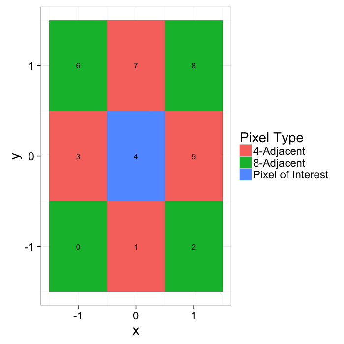
Formal Neighborhood Definitions
Formally these have two effectively equivalent, but different definitions.
- Pixels which share a face (red line) with the pixel
- Pixels which share a vertex (yellow dot) with the pixel
cent.pix<-data.frame(x=c(-1, 1,1,-1,-1)/2,
y=c(-1,-1,1, 1,-1)/2)
ggplot(morph.2d,aes(x=x,y=y))+
geom_tile(color="black",size=1,alpha=0.7,
aes(fill=ifelse(r==0,"Pixel of Interest",
ifelse(r==1,"4-Adjacent","8-Adjacent")))
)+
geom_path(data=cent.pix,color="red",size=3)+
geom_point(data=cent.pix,color="yellow",size=5)+
geom_text(aes(label=3*(y+1)+x+1))+
labs(fill="Pixel Type")+
theme_bw(20)
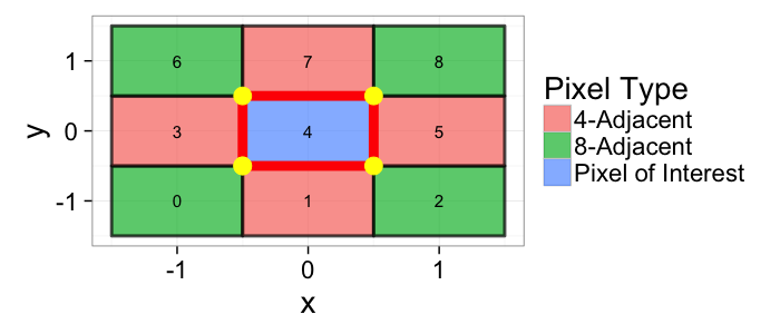
- Pixels which are distance 1 from the pixel
- Pixels which are distance $\sqrt{2}$ from the pixel
morph.2d<-expand.grid(x=c(-1,0,1),y=c(-1,0,1))
morph.2d$r<-with(morph.2d,sqrt(x^2+y^2))
ggplot(morph.2d,aes(x=x,y=y))+
geom_tile(color="black",
aes(fill=ifelse(r==0,"Pixel of Interest",
ifelse(r==1,"4-Adjacent","8-Adjacent")))
)+
geom_text(aes(label=round(r*100)/100))+
labs(fill="Pixel Type")+
theme_bw(20)
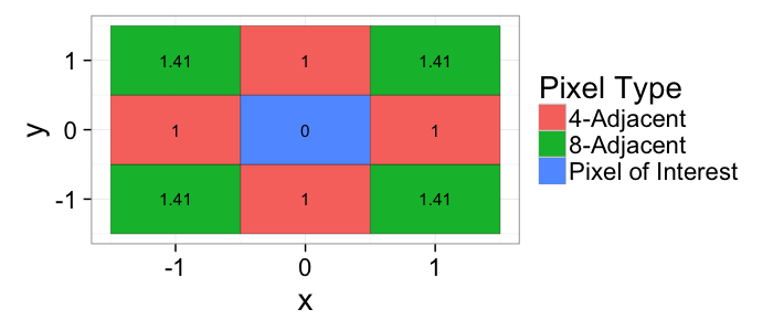
Formal Neighborhood Definitions in 3D
In 3D there is now an additional group to consider because of the extra-dimension
- Voxels which share a face (red line) with the voxel (6-adjacent)
- Voxels which share an edge (yellow dot) with the voxel (18-adjacent)
- Voxels which share a vertex (purple dot) with the voxel (26-adjacent)
morph.3d<-expand.grid(x=c(-1,0,1),y=c(-1,0,1),z=c(-1,0,1))
morph.3d$r<-with(morph.3d,sqrt(x^2+y^2+z^2))
cent.pix.3d<-data.frame(x=c(-1, 1,1,-1,-1,-1, 1,1,-1,-1)/2,
y=c(-1,-1,1, 1,-1,-1,-1,1, 1,-1)/2,
z=c(-1,-1,-1,-1,-1,1, 1,1, 1, 1))
face.pix.3d<-data.frame(x=c(-1, 1, 1,-1,-1)/2,
y=c(-1,-1, 1, 1,-1)/2,
z=c( 0, 0, 0, 0, 0))
pixel.label<-function(r) ifelse(r==0,"Pixel of Interest",
ifelse(r==1," 6-Adjacent",
ifelse(r==sqrt(2),"18-Adjacent","26-Adjacent")))
ggplot(morph.3d,aes(x=x,y=y))+
geom_tile(color="black",size=1,alpha=0.7,
aes(fill=pixel.label(r))
)+
geom_path(data=cent.pix.3d,color="yellow",size=3)+
geom_point(data=cent.pix.3d,color="purple",size=5)+
geom_path(data=face.pix.3d,color="red",size=3)+
geom_point(data=face.pix.3d,color="yellow",size=5)+
geom_text(aes(label=9*(z+1)+3*(y+1)+x+1))+
facet_grid(~z)+
labs(fill="Pixel Type")+
theme_bw(20)
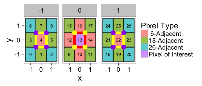
- Voxels which are distance 1 from the voxel
- Voxels which are distance $\sqrt{2}$ from the voxel
- Voxels which are distance $\sqrt{3}$ from the voxel
ggplot(morph.3d,aes(x=x,y=y))+
geom_tile(color="black",size=1,
aes(fill=pixel.label(r))
)+
geom_text(aes(label=round(r*100)/100))+
facet_grid(~z)+
labs(fill="Pixel Type")+
theme_bw(14)
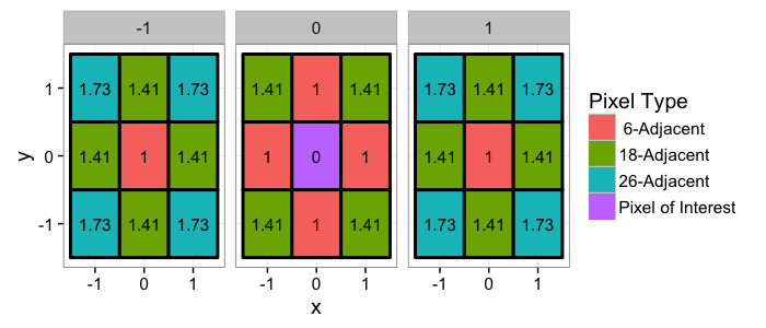
Erosion and Dilation
Erosion
If any of the voxels in the neighborhood are 0/false than the voxel will be set to 0
- Has the effect of peeling the surface layer off of an object
Dilation
If any of the voxels in the neigbhorhood are 1/true then the voxel will be set to 1
- Has the effect of adding a layer onto an object (dunking an strawberry in chocolate, adding a coat of paint to a car)
Applied Erosion and Dilation
Dilation
Taking an image of the cross at a too-high threshold, we show how dilation can be used to recover some of the missing pixels
cross.im$thresh<-cross.im$col>1.75
cross.mat<-df.to.im(cross.im,"thresh",inv=T)
cross.df<-im.to.df(cross.mat)
ggplot(cross.df,aes(x=x,y=y))+
geom_tile(data=subset(cross.df,val==0),aes(fill="original"),color="black",alpha=0.7)+
labs(fill="Type")+
theme_bw(20)

cross.dil.mat<-erode(cross.mat,makeBrush(3,shape = 'box'))
cross.dil.df<-im.to.df(cross.dil.mat)
ggplot(cross.df,aes(x=x,y=y))+
geom_tile(data=subset(cross.df,val==0),aes(fill="original"),color="black",alpha=0.7)+
geom_tile(data=subset(cross.dil.df,val==0),aes(fill="post dilation"),color="black",alpha=0.3)+
labs(fill="Type")+
theme_bw(20)

Erosion
Taking an image of the cross at a too-low threshold, we show how erosion can be used to remove some of the extra pixels
cross.im$thresh<-cross.im$col>0.4
cross.mat<-df.to.im(cross.im,"thresh",inv=T)
cross.df<-im.to.df(cross.mat)
ggplot(cross.df,aes(x=x,y=y))+
geom_tile(data=subset(cross.df,val==0),aes(fill="original"),color="black",alpha=0.7)+
labs(fill="Type")+
theme_bw(20)

cross.ero.mat<-dilate(cross.mat,makeBrush(3,shape = 'box'))
cross.ero.df<-im.to.df(cross.ero.mat)
ggplot(cross.df,aes(x=x,y=y))+
geom_tile(data=subset(cross.df,val==0),aes(fill="original"),color="black",alpha=0.7)+
geom_tile(data=subset(cross.ero.df,val==0),aes(fill="post erosion"),color="black",alpha=0.3)+
labs(fill="Type")+
theme_bw(20)

Opening and Closing
Opening
An erosion followed by a dilation operation
- Peels a layer off and adds a layer on
- Very small objects and connections are deleted in the erosion and do not return the image is thus __open__ed
- A cube larger than several voxels will have the exact same volume after (conservative)
Closing
A dilation followed by an erosion operation
- Adds a layer and then peels a layer off
- Objects that are very close are connected when the layer is added and they stay connected when the layer is removed thus the image is __close__d
- A cube larger than one voxel will have the exact same volume after (conservative)
Applied Opening and Closing
Opening
Taking an image of the cross at a too-low threshold, we show how opening can be used to remove some of the extra pixels
cross.im$thresh<-cross.im$col>0.4
cross.mat<-df.to.im(cross.im,"thresh",inv=T)
cross.df<-im.to.df(cross.mat)
ggplot(cross.df,aes(x=x,y=y))+
geom_tile(data=subset(cross.df,val==0),aes(fill="original"),color="black",alpha=0.7)+
labs(fill="Type")+
theme_bw(20)

cross.ero.mat<-closing(cross.mat,makeBrush(3,'box'))
cross.ero.df<-im.to.df(cross.ero.mat)
ggplot(cross.df,aes(x=x,y=y))+
geom_tile(data=subset(cross.df,val==0),aes(fill="original"),color="black",alpha=0.7)+
geom_tile(data=subset(cross.ero.df,val==0),aes(fill="post opening"),color="black",alpha=0.3)+
labs(fill="Type")+
theme_bw(20)

Closing
Taking an image of the cross at a too-high threshold, we show how closing can be used to recover some of the missing pixels
cross.im$thresh<-cross.im$col>1.6
cross.mat<-df.to.im(cross.im,"thresh",inv=T)
cross.df<-im.to.df(cross.mat)
ggplot(cross.df,aes(x=x,y=y))+
geom_tile(data=subset(cross.df,val==0),aes(fill="original"),color="black",alpha=0.7)+
labs(fill="Type")+
theme_bw(20)

cross.dil.mat<-opening(cross.mat,makeBrush(3,'box'))
cross.dil.df<-im.to.df(cross.dil.mat)
ggplot(cross.df,aes(x=x,y=y))+
geom_tile(data=subset(cross.df,val==0),aes(fill="original"),color="black",alpha=0.7)+
geom_tile(data=subset(cross.dil.df,val==0),aes(fill="post closing"),color="black",alpha=0.3)+
labs(fill="Type")+
theme_bw(20)

Applying Morphological Tools
- For many applications morphology appears to be the same as filter
- The key difference is the avalanche or non-linear nature of the results
- A single off voxel can turn its entire neighborhood off (erosion)
- A single on voxel can turn its entire neighborhood on (dilation)
- The effects of this are most pronounced when performed iteratively
- This is very useful for filling holes, connecting objects, creating masks
A segmented slice taken from a cortical bone sample. The dark is the calcified bone tissue and the white are holes in the image

Filling Holes / Creating Masks
cortbone.im<-png::readPNG("ext-figures/bone.png") %>% t
cortbone.df<-im.to.df(cortbone.im)
#cortbone.df$val<-255*(cortbone.df$val>0.5)
cortbone.close.im<-opening(cortbone.im,makeBrush(3,'box'))
ggplot(subset(cortbone.df,val<1),aes(x=x,y=518-y))+
geom_raster(data=subset(im.to.df(cortbone.close.im),val<1),
aes(fill="closing 3x3"),alpha=0.8)+
geom_raster(aes(fill="before closing"),alpha=0.6)+
labs(fill="Image",y="y",x="x",title="3x3 Closing")+
coord_equal()+
theme_bw(20)

cortbone.close.im<-opening(cortbone.im,makeBrush(7,'box'))
ggplot(subset(cortbone.df,val<1),aes(x=x,y=600-y))+
geom_raster(data=subset(im.to.df(cortbone.close.im),val<1),
aes(fill="closing 7x7"),alpha=0.8)+
geom_raster(aes(fill="before closing"),alpha=0.6)+
labs(fill="Image",y="y",x="x",title="7x7 Closing")+
coord_equal()+
theme_bw(20)

Filling Holes / Creating Masks
Applying the closing with even larger windows will close everything but being to destroy the underlying structure of the mask
full.kernel<-makeBrush(45,"box")
cortbone.close.im<-closing(cortbone.im<1,full.kernel)
## Error in is(y, "Image"): object 'cortbone.im' not found
ggplot(subset(cortbone.df,val<1),aes(x=x,y=600-y))+
geom_raster(data=subset(im.to.df(cortbone.close.im),val>0),
aes(fill="closing 45x45"),alpha=0.8)+
geom_raster(aes(fill="before closing"),alpha=0.6)+
labs(fill="Image",y="x",x="y",title="45x45 Closing")+
coord_equal()+
theme_bw(20)
## Error in subset(cortbone.df, val < 1): object 'cortbone.df' not found
We can characterize this by examining the dependency of the closing size and the volume fraction (note scale)
get.vf<-function(img) (100*sum(img>0)/
(nrow(cortbone.im)*ncol(cortbone.im)))
vf.of.closing<-function(dim.size) {
data.frame(dim.size=dim.size,
vf.full=get.vf(closing(cortbone.im<1,makeBrush(dim.size,"box" )))
)
}
pt.list<-c(seq(1,10),seq(11,40,2))
vf.df<-ldply(pt.list,vf.of.closing,.parallel=T)
## Error in do.ply(i): task 1 failed - "object 'cortbone.im' not found"
ggplot(vf.df,aes(x=dim.size))+
geom_line(aes(y=vf.full))+
labs(fill="Image",y="Bone Volume Frac(%)",x="Closing Size",title="Closing Size vs Volume Fraction")+
theme_bw(15)
## Error in ggplot(vf.df, aes(x = dim.size)): object 'vf.df' not found
- Be careful when using large area opening / closing operations (always check the images)
- Noise and defects in images can be amplified with these larger operations
Different Kernels
Using a better kernel shape (circular, diamond shaped, etc) the artifacts from morphological operations can be reduced
disc.kernel<-makeBrush(45,"disc")
cortbone.close.im<-closing(cortbone.im<1,disc.kernel)
## Error in is(y, "Image"): object 'cortbone.im' not found
ggplot(subset(cortbone.df,val<1),aes(x=x,y=600-y))+
geom_raster(data=subset(im.to.df(cortbone.close.im),val>0),
aes(fill="closing 45x45"),alpha=0.8)+
geom_raster(aes(fill="before closing"),alpha=0.6)+
labs(fill="Image",y="x",x="y",title="45x45 Closing")+
coord_equal()+
theme_bw(20)
## Error in subset(cortbone.df, val < 1): object 'cortbone.df' not found
We can characterize this by examining the dependency of the closing size and the volume fraction (note scale)
get.vf<-function(img) (100*sum(img>0)/
(nrow(cortbone.im)*ncol(cortbone.im)))
vf.of.closing<-function(dim.size) {
data.frame(dim.size=dim.size,
vf.full=get.vf(closing(cortbone.im<1,makeBrush(dim.size,"box" ))),
vf.disc=get.vf(closing(cortbone.im<1,makeBrush(dim.size,"disc"))),
vf.diam=get.vf(closing(cortbone.im<1,makeBrush(dim.size,"diamond"))),
vf.vline=get.vf(closing(cortbone.im<1,makeBrush(dim.size,"line",angle=0))),
vf.hline=get.vf(closing(cortbone.im<1,makeBrush(dim.size,"line",angle=90)))
)
}
pt.list<-c(seq(1,9,2),seq(11,60,4))
vf.df<-ldply(pt.list,vf.of.closing,.parallel=T)
## Error in do.ply(i): task 1 failed - "object 'cortbone.im' not found"
ggplot(vf.df,aes(x=dim.size))+
geom_line(aes(y=vf.full,color="Full"))+
geom_line(aes(y=vf.disc,color="Circular"))+
geom_line(aes(y=vf.diam,color="Diamond-Shape"))+
geom_line(aes(y=vf.vline,color="Vertical Line"))+
geom_line(aes(y=vf.hline,color="Horizontal Line"))+
labs(color="Kernel Used",y="Bone Volume Fraction (%)",x="Closing Size",title="Closing Size vs Volume Fraction")+
theme_bw(20)
## Error in ggplot(vf.df, aes(x = dim.size)): object 'vf.df' not found
- Alternative techniques
- Convex Hull - assuming convex shapes
- Flood Filling - fill connected pixels like in Microsoft Paint
Segmenting Fossils
Taken from the BBC Documentary First Life by David Attenborough
- Gut Data
- Slice 182 you can make out the intenstine track
- Teeth Data
- Explore the sample and apply a threshold to locate the teeth using the 3D viewer
Quantifying Alzheimers: Segment the Cortex
Courtesy of Alberto Alfonso
- Understand the progress of Alzheimer’s disease as it relates to plaque formation in different regions of the brain
- First identify different regions
- Manually contoured

Quantifying Alzheimers: Segment the Cortex
- The cortex is barely visible to the human eye
- Tiny structures hint at where cortex is located
alz.df<-im.to.df(t(png::readPNG("ext-figures/cortex.png")))
ggplot(alz.df,aes(x=x,y=518-y))+
geom_raster(aes(fill=val))+
labs(fill="Electron Density",y="y",x="x")+
coord_equal()+
theme_bw(20)

- A simple threshold is insufficient to finding the cortical structures
- Other filtering techniques are unlikely to magicially fix this problem
ggplot(alz.df,aes(x=x,y=518-y))+
geom_raster(aes(fill=cut_interval(val,4)))+
labs(fill="Segmented Phases",y="y",x="x")+
coord_equal()+
theme_bw(20)

Surface Area / Perimeter
We see that the dilation and erosion affects are strongly related to the surface area of an object: the more surface area the larger the affect of a single dilation or erosion step.
make.circle<-function(nx,r,nscale=1) {
ny<-nx
grad.im<-expand.grid(x=c(-nx:nx)/nscale,y=c(-ny:ny)/nscale)
grad.im$val<-with(grad.im,(x^2+y^2)

calc.eros.cnt<-function(nx,r,nscale=1,im.fun=make.circle) {
in.cir<-im.fun(nx,r,nscale=nscale)
cir.im<-df.to.im(in.cir)
data.frame(nx=nx,r=r,nscale=nscale,
dvolume=sum(dilate(cir.im>0,makeBrush(3,"diamond"))>0),
evolume=sum(erode(cir.im>0,makeBrush(3,"diamond"))>0),
volume=sum(cir.im>0)
)
}
max.rad<-20
r.list<-seq(0.2,max.rad,length.out=20)
r.table<-ldply(r.list,function(r) calc.eros.cnt(max.rad+1,r,1))
r.table$model.perimeter<-with(r.table,2*pi*r)
r.table$estimated.perimeter<-with(r.table,
((dvolume-volume)+(volume-evolume))/2)
ggplot(r.table,aes(x=r))+
geom_line(aes(y=estimated.perimeter,color="Morphological Estimation"))+
geom_line(aes(y=model.perimeter,color="Model Circumference"))+
labs(x="Radius",y="Perimeter",color="Source")+
theme_bw(20)
