## Loading required package: knitr
require(ggplot2)
require(lattice) # nicer scatter plots
require(plyr)
require(grid) # contains the arrow function
require(biOps)
require(doMC) # for parallel code
require(EBImage)
require(reshape2) # for the melt function
## To install EBImage
# source("http://bioconductor.org/biocLite.R")
# biocLite("EBImage")

# start parallel environment
registerDoMC()
# functions for converting images back and forth
im.to.df<-function(in.img) {
  out.im<-expand.grid(x=1:nrow(in.img),y=1:ncol(in.img))
  out.im$val<-as.vector(in.img)
  out.im
  }
df.to.im<-function(in.df,val.col="val",inv=F) {
  in.vals<-in.df[[val.col]]
  if(class(in.vals[1])=="logical") in.vals<-as.integer(in.vals*255)
  if(inv) in.vals<-255-in.vals
  out.mat<-matrix(in.vals,nrow=length(unique(in.df$x)),byrow=F)
  attr(out.mat,"type")<-"grey"
  out.mat
  }
ddply.cutcols<-function(...,cols=1) {
  # run standard ddply command
  cur.table<-ddply(...)
  cutlabel.fixer<-function(oVal) {
    sapply(oVal,function(x) {
      cnv<-as.character(x)
      mean(as.numeric(strsplit(substr(cnv,2,nchar(cnv)-1),",")[[1]]))
      })
    }
  cutname.fixer<-function(c.str) {
    s.str<-strsplit(c.str,"(",fixed=T)[[1]]
    t.str<-strsplit(paste(s.str[c(2:length(s.str))],collapse="("),",")[[1]]
    paste(t.str[c(1:length(t.str)-1)],collapse=",")
    }
  for(i in c(1:cols)) {
    cur.table[,i]<-cutlabel.fixer(cur.table[,i])
    names(cur.table)[i]<-cutname.fixer(names(cur.table)[i])
    }
  cur.table
  }
## Standard image processing tools which I use for visualizing the examples in the script
commean.fun<-function(in.df) {
  ddply(in.df,.(val), function(c.cell) {
    weight.sum<-sum(c.cell$weight)
    data.frame(xv=mean(c.cell$x),
               yv=mean(c.cell$y),
               xm=with(c.cell,sum(x*weight)/weight.sum),
               ym=with(c.cell,sum(y*weight)/weight.sum)
               )
    })
  }

colMeans.df<-function(x,...) as.data.frame(t(colMeans(x,...)))

pca.fun<-function(in.df) {
  ddply(in.df,.(val), function(c.cell) {
    c.cell.cov<-cov(c.cell[,c("x","y")])
    c.cell.eigen<-eigen(c.cell.cov)

    c.cell.mean<-colMeans.df(c.cell[,c("x","y")])
    out.df<-cbind(c.cell.mean,
                  data.frame(vx=c.cell.eigen$vectors[1,],
                             vy=c.cell.eigen$vectors[2,],
                             vw=sqrt(c.cell.eigen$values),
                             th.off=atan2(c.cell.eigen$vectors[2,],c.cell.eigen$vectors[1,]))
                  )
    })
  }
vec.to.ellipse<-function(pca.df) {
  ddply(pca.df,.(val),function(cur.pca) {
    # assume there are two vectors now
    create.ellipse.points(x.off=cur.pca[1,"x"],y.off=cur.pca[1,"y"],
                          b=sqrt(5)*cur.pca[1,"vw"],a=sqrt(5)*cur.pca[2,"vw"],
                          th.off=pi/2-atan2(cur.pca[1,"vy"],cur.pca[1,"vx"]),
                          x.cent=cur.pca[1,"x"],y.cent=cur.pca[1,"y"])
    })
  }

# test function for ellipse generation
# ggplot(ldply(seq(-pi,pi,length.out=100),function(th) create.ellipse.points(a=1,b=2,th.off=th,th.val=th)),aes(x=x,y=y))+geom_path()+facet_wrap(~th.val)+coord_equal()
create.ellipse.points<-function(x.off=0,y.off=0,a=1,b=NULL,th.off=0,th.max=2*pi,pts=36,...) {
  if (is.null(b)) b<-a
  th<-seq(0,th.max,length.out=pts)
  data.frame(x=a*cos(th.off)*cos(th)+b*sin(th.off)*sin(th)+x.off,
             y=-1*a*sin(th.off)*cos(th)+b*cos(th.off)*sin(th)+y.off,
             id=as.factor(paste(x.off,y.off,a,b,th.off,pts,sep=":")),...)
  }
deform.ellipse.draw<-function(c.box) {
  create.ellipse.points(x.off=c.box$x[1],
                        y.off=c.box$y[1],
                        a=c.box$a[1],
                        b=c.box$b[1],
                        th.off=c.box$th[1],
                        col=c.box$col[1])
  }
bbox.fun<-function(in.df) {
  ddply(in.df,.(val), function(c.cell) {
    c.cell.mean<-colMeans.df(c.cell[,c("x","y")])
    xmn<-emin(c.cell$x)
    xmx<-emax(c.cell$x)
    ymn<-emin(c.cell$y)
    ymx<-emax(c.cell$y)
    out.df<-cbind(c.cell.mean,
                  data.frame(xi=c(xmn,xmn,xmx,xmx,xmn),
                             yi=c(ymn,ymx,ymx,ymn,ymn),
                             xw=xmx-xmn,
                             yw=ymx-ymn
                             ))
    })
  }

# since the edge of the pixel is 0.5 away from the middle of the pixel
emin<-function(...) min(...)-0.5
emax<-function(...) max(...)+0.5
extents.fun<-function(in.df) {
  ddply(in.df,.(val), function(c.cell) {
    c.cell.mean<-colMeans.df(c.cell[,c("x","y")])
    out.df<-cbind(c.cell.mean,data.frame(xmin=c(c.cell.mean$x,emin(c.cell$x)),
                                         xmax=c(c.cell.mean$x,emax(c.cell$x)),
                                         ymin=c(emin(c.cell$y),c.cell.mean$y),
                                         ymax=c(emax(c.cell$y),c.cell.mean$y)))
    })
  }

th_fillmap.fn<-function(max.val) scale_fill_gradientn(colours=rainbow(10),limits=c(0,max.val))
Quantitative Big Imaging
author: Kevin Mader
date: 3 April 2014
width: 1440
height: 900
css: ../template.css
transition: rotate
ETHZ: 227-0966-00L
Many Objects and Distributions
Course Outline
- 20th February - Introductory Lecture
- 27th February - Filtering and Image Enhancement (A. Kaestner)
- 6th March - Basic Segmentation, Discrete Binary Structures
- 13th March - Advanced Segmentation
- 20th March - Analyzing Single Objects
- 27th March - Analyzing Complex Objects
- 3rd April - Many Objects and Distributions
- 10th April - Statistics and Reproducibility
- 17th April - Dynamic Experiments
- 8th May - Big Data
- 15th May - Guest Lecture - In-Operando Imaging of Batteries (V. Wood)
- 22th May - Project Presentations
Literature / Useful References
Books
- Jean Claude, Morphometry with R
- John C. Russ, “The Image Processing Handbook”,(Boca Raton, CRC Press)
- Available online within domain ethz.ch (or proxy.ethz.ch / public VPN)
- J. Weickert, Visualization and Processing of Tensor Fields
Papers / Sites
Previously on QBI ...
- Image Enhancment
- Highlighting the contrast of interest in images
- Minimizing Noise
- Understanding image histograms
- Automatic Methods
- Component Labeling
- Single Shape Analysis
- Complicated Shapes
Outline
- Motivation (Why and How?)
- Local Environment
- Neighbors
- Voronoi Tesselation
- Distribution Tensor
- Global Enviroment
- Alignment
- Self-Avoidance
- Two Point Correlation Function
What do we start with?
Going back to our original cell image
- We have been able to get rid of the noise in the image and find all the cells (lecture 2-4)
- We have analyzed the shape of the cells using the shape tensor (lecture 5)
- We even separated cells joined together using Watershed (lecture 6)
We can characterize the sample and the average and standard deviations of volume, orientation, surface area, and other metrics
Motivation (Why and How?)
With all of these images, the first step is always to understand exactly what we are trying to learn from our images.
cell.im<-jpeg::readJPEG("ext-figures/Cell_Colony.jpg")
cell.lab.df<-im.to.df(bwlabel(cell.im<.6))
size.histogram<-ddply(subset(cell.lab.df,val>0),.(val),function(c.label) data.frame(count=nrow(c.label)))
keep.vals<-subset(size.histogram,count>25)


cur.cell.df<-subset(cell.lab.df,val %in% keep.vals$val)
cell.pca<-pca.fun(cur.cell.df)
cell.ellipse<-vec.to.ellipse(cell.pca)
ggplot(cur.cell.df,aes(x=x,y=y))+
  geom_tile(color="black",fill="grey")+
  geom_path(data=cell.ellipse,aes(color="Ellipse",group=val))+
  geom_path(data=bbox.fun(cur.cell.df),aes(x=xi,y=yi,color="Bounding\nBox",group=val))+
  labs(title="Single Cell",color="Shape\nAnalysis\nMethod")+
  theme_bw(20)+coord_equal()+guides(fill=F)
We want to know how many cells are alive
- Maybe small cells are dead and larger cells are alive \(\rightarrow\) examine the volume distribution
- Maybe living cells are round and dead cells are really spiky and pointy \(\rightarrow\) examine anisotropy
We want to know where the cells are alive or most densely packed
- We can visually inspect the sample (maybe even color by volume)
- We can examine the raw positions (x,y,z) but what does that really tell us?
- We can make boxes and count the cells inside each one
- How do we compare two regions in the same sample or even two samples?
Motivation (continued)
ggplot(cur.cell.df,aes(x=x,y=y))+
  geom_tile(color="black",fill="grey")+
  geom_path(data=cell.ellipse,aes(color="Ellipse",group=val))+
  geom_path(data=bbox.fun(cur.cell.df),aes(x=xi,y=yi,color="Bounding\nBox",group=val))+
  labs(title="Single Cell",color="Shape\nAnalysis\nMethod")+
  theme_bw(20)+coord_equal()+guides(fill=F)
- We want to know how the cells are communicating
- Maybe physically connected cells (touching) are communicating \(\rightarrow\) watershed
- Maybe cells oriented the same direction are communicating \(\rightarrow\) average? orientation
- Maybe cells which are close enough are communicating \(\rightarrow\) ?
- Maybe cells form hub and spoke networks \(\rightarrow\) ?
Motivation (continued)
ggplot(cur.cell.df,aes(x=x,y=y))+
  geom_tile(color="black",fill="grey")+
  geom_path(data=cell.ellipse,aes(color="Ellipse",group=val))+
  geom_path(data=bbox.fun(cur.cell.df),aes(x=xi,y=yi,color="Bounding\nBox",group=val))+
  labs(title="Single Cell",color="Shape\nAnalysis\nMethod")+
  theme_bw(20)+coord_equal()+guides(fill=F)
- We want to know how the cells are nourished
- Maybe closely packed cells are better nourished \(\rightarrow\) count cells in a box?
- Maybe cells are oriented around canals which supply them \(\rightarrow\) ?
So what do we still need
- A way for counting cells in a region and estimating density without creating arbitrary boxes
- A way for finding out how many cells are near a given cell, it's nearest neighbors
- A way for quantifying how far apart cells are and then comparing different regions within a sample
- A way for quantifying and comparing orientations
- the mean of 0\(^\circ\) and 180\(^\circ\) = 90\(^\circ\)
- the distance between -180\(^\circ\) and 179\(^\circ\) is 359\(^\circ\)
- since we have not defined a tip or head, 0\(^\circ\) and 180\(^\circ\) are actually the same
What would be really great?
A tool which could be adapted to answering a large variety of problems
- multiple types of structures
- multiple phases
Destructive Measurements
With most imaging techniques and sample types, the task of measurement itself impacts the sample.
- Even techniques like X-ray tomography which claim to be non-destructive still impart significant to lethal doses of X-ray radition for high resolution imaging
- Electron microscopy, auto-tome-based methods, histology are all markedly more destructive and make longitudinal studies impossible
- Even when such measurements are possible
- Registration can be a difficult task and introduce artifacts
Why is this important?
- techniques which allow us to compare different samples of the same type.
- are sensitive to common transformations
- Sample B after the treatment looks like Sample A stretched to be 2x larger
- The volume fraction at the center is higher than the edges but organization remains the same
Ok, so now what?
ggplot(cur.cell.df,aes(x=x,y=y))+
  geom_tile(color="black",fill="grey")+
  geom_path(data=cell.ellipse,aes(color="Ellipse",group=val))+
  labs(title="Zoomed into a smaller region")+
  xlim(200,400)+ylim(100,300)+
  theme_bw(20)+coord_equal()+guides(fill=F,color=F)
\[ \downarrow \]
kable(head(cell.pca[,c("x","y","vx","vy")]),align='c',digits=2)
| x |
y |
vx |
vy |
| 20.19 |
10.69 |
-0.95 |
-0.30 |
| 20.19 |
10.69 |
0.30 |
-0.95 |
| 293.08 |
13.18 |
-0.50 |
0.86 |
| 293.08 |
13.18 |
-0.86 |
-0.50 |
| 243.81 |
14.23 |
0.68 |
0.74 |
| 243.81 |
14.23 |
-0.74 |
0.68 |
\[ \cdots \]
So if we want to know the the mean or standard deviations of the position or orientations we can analyze them easily.
cell.pca$Theta<-cell.pca$th.off*180/pi
cell.pca$Length<-cell.pca$vw
s.table<-apply(cell.pca[,c("x","y","Length","vx","vy","Theta")],2,summary)

kable(t(s.table),align='c',digits=2)
| id |
Min. |
1st Qu. |
Median |
Mean |
3rd Qu. |
Max. |
| x |
6.90 |
216.00 |
281.00 |
258.00 |
339.00 |
406.00 |
| y |
10.70 |
112.00 |
221.00 |
209.00 |
313.00 |
395.00 |
| Length |
1.06 |
1.57 |
1.95 |
2.08 |
2.41 |
4.32 |
| vx |
-1.00 |
-0.94 |
-0.70 |
-0.42 |
0.07 |
0.71 |
| vy |
-1.00 |
-0.70 |
0.02 |
0.04 |
0.71 |
1.00 |
| Theta |
-180.00 |
-134.00 |
-0.50 |
-4.67 |
131.00 |
178.00 |
- But what if we want more or other information?
Calculating Density
One of the first metrics to examine with distribution is density \(\rightarrow\) how many objects in a given region or volume.
It is deceptively easy to calculate involving the ratio of the number of objects divided by the volume.
pt.maker<-function(n.pts,rn.fun=function(pts) runif(pts,min=0,max=1),...) data.frame(x=rn.fun(n.pts),y=rn.fun(n.pts),n.pts=n.pts,...)

ggplot(ldply(c(10,100,1000),pt.maker),aes(x,y))+
  geom_point()+facet_grid(n.pts~.)+
  coord_equal()+
  theme_bw(20)
It doesn't tell us much, many very different systems with the same density and what if we want the density of a single point? Does that even make sense?
dist.funs<-c(function(pts) runif(pts,min=0,max=1),
             function(pts) rnorm(pts,mean=0.5,sd=0.3),
             function(pts) rnorm(pts,mean=0.5,sd=0.1),
             function(pts) rlnorm(pts,meanlog=1.5,sdlog=1.5)/exp(3))

ggplot(ldply(1:length(dist.funs),function(fun.ind) pt.maker(500,rn.fun=dist.funs[[fun.ind]],fun.ind=fun.ind)),
       aes(x,y))+
  geom_point()+facet_grid(fun.ind~.)+
  coord_equal()+
  xlim(0,1.01)+ylim(0,1.01)+
  labs(title="Density = 500 N/mm^2")+
  theme_bw(20)
Neighbors
Definition
Oxford American \(\rightarrow\) be situated next to or very near to (another)
- Does not sound very scientific
- How close?
- Touching, closer than anything else?
Nearest Neighbor (distance)
find.nn<-function(in.df) {
  ddply(in.df,.(val),function(c.group) {
    cur.val<-c.group$val[1]
    cur.x<-c.group$x[1]
    cur.y<-c.group$y[1]
    all.butme<-subset(in.df,val!=cur.val)
    all.butme$dist<-with(all.butme,sqrt((x-cur.x)^2+(y-cur.y)^2))
    min.ele<-subset(all.butme,dist<=min(all.butme$dist))
    min.ele.order<-order(runif(nrow(min.ele)))
    min.ele<-min.ele[min.ele.order,]
    out.df<-data.frame(x=cur.x,y=cur.y,
               xe=min.ele$x[1],ye=min.ele$y[1],vale=min.ele$val[1],dist=min.ele$dist[1])
    out.df
    })
}
Given a set of objects with centroids at
\[ \textbf{P}=\begin{bmatrix} \vec{x}_0,\vec{x}_1,\cdots,\vec{x}_i \end{bmatrix} \]
We can define the nearest neighbor as the position of the object in our set which is closest
\[ \vec{\textrm{NN}}(\vec{y}) = \textrm{argmin}(||\vec{y}-\vec{x}|| \forall \vec{x} \in \textbf{P}-\vec{y}) \]
We define the distance as the Euclidean distance from the current point to that point, and the angle as the
\[ \textrm{NND}(\vec{y}) = \textrm{min}(||\vec{y}-\vec{x}|| \forall \vec{x} \in \textbf{P}-\vec{y}) \]
\[ \textrm{NN}\theta(\vec{y}) = \tan^{-1}\frac{(\vec{\textrm{NN}}-\vec{y})\cdot \vec{j}}{(\vec{\textrm{NN}}-\vec{y})\cdot \vec{i}} \]
Nearest Neighbor Definition
So examining a simple starting system like a grid, we already start running into issues.
- In a perfect grid like structure each object has 4 equidistant neighbors (6 in 3D)
- Which one is closest?
We thus add an additional clause (only relevant for simulated data) where if there are multiple equidistant neighbors, a nearest is chosen randomly
This ensures when we examine the orientation distribution (NN\(\theta\)) of the neighbors it is evenly distributed
cur.grid<-expand.grid(x=-c(-4:4),y=c(-4:4))
cur.grid$val<-1:nrow(cur.grid)
std.grid<-cur.grid
ggplot(cur.grid,aes(x=x,y=y))+
  geom_segment(data=find.nn(cur.grid),aes(xend=xe,yend=ye),
               arrow=arrow(length = unit(0.3,"cm")),alpha=0.75)+
  geom_point(aes(color=val),size=3,alpha=0.75)+
  labs(title="Single Cell",color="Label")+
  scale_color_gradientn(colours=rainbow(10))+
  coord_equal()+
  theme_bw(20)+guides(fill=F)
In-Silico Systems
For the rest of these sections we will repeatedly use several simple in-silico systems to test our methods and try to better understand the kind of results we obtain from them.
Compression
- The most simple system simply involves a scaling in every direction by \(\alpha\)
- \(\alpha<1\) the system is compressed
- \(\alpha>1\) the system is expanded
\[ \begin{bmatrix} x^\prime \\ y^\prime \end{bmatrix} = \alpha \begin{bmatrix} x \\ y \end{bmatrix} \]
Shearing
- Slightly more complicated system where objects are shifted based on their location using a slope of \(\alpha\)
\[ \begin{bmatrix} x^\prime \\ y^\prime \end{bmatrix} = \begin{bmatrix} 1 & \alpha \\ 0 & 1 \end{bmatrix} \begin{bmatrix} x \\ y \end{bmatrix} \]
In-Silico Systems (Continued)
- Stretch
- A non-evenly distributed system with a parameter \(\alpha\) controlling if objects bunch near the edges or the center. A maximum distance \(m\) is defined as the magnitude of the largest offset in x or y
- + Same total volume just arranged differently
\[ \begin{bmatrix} x^\prime \\ y^\prime \end{bmatrix} = \begin{bmatrix} \textrm{sign}(x) \left(\frac{|x|}{m}\right)^\alpha m \\ \textrm{sign}(y) \left(\frac{|y|}{m}\right)^\alpha m \end{bmatrix} \]
- Swirl
- A transformation where the points are rotated more based on how far away they are from the center and the slope of the swirl (\(\alpha\)),
\[ \theta (x,y) = \alpha \sqrt{x^2+y^2} \]
\[ \begin{bmatrix} x^\prime \\ y^\prime \end{bmatrix} =
\begin{bmatrix} \cos\theta(x,y) & -\sin\theta(x,y) \\
\sin\theta(x,y) & \cos\theta(x,y)
\end{bmatrix} \begin{bmatrix} x \\ y \end{bmatrix} \]
Examining Compression
comp.fun<-function(c.stretch,in.grid=cur.grid) {
  str.grid<-in.grid
  str.grid$x<-with(in.grid,c.stretch*x)
  str.grid$y<-with(in.grid,c.stretch*y)
  cbind(str.grid,glab=c.stretch)
}
test.systems.comp<-ldply(c(0.8,1,1.2),comp.fun)

dist.plots.comp<-ddply(test.systems.comp,.(glab),find.nn)
ggplot(test.systems.comp,aes(x=x,y=y))+
  geom_segment(data=dist.plots.comp,aes(xend=xe,yend=ye),
               arrow=arrow(length = unit(0.3,"cm")),alpha=0.75)+
  geom_point(aes(color=val),size=3,alpha=0.75)+
  labs(title="Positions and Neighbors",color="Label")+
  scale_color_gradientn(colours=rainbow(10))+
    coord_equal()+
  facet_grid(glab~.)+
  theme_bw(20)
ggplot(dist.plots.comp,
       aes(x=0,y=0,xend=xe-x,yend=ye-y))+
    geom_density2d(aes(x=xe-x,y=ye-y),color="red",alpha=0.7)+
  geom_segment(aes(color=glab),
               arrow=arrow(length = unit(0.3,"cm")))+
  facet_grid(glab~.)+
    coord_equal()+
  labs(title="Nearest Neighbor Orientations")+guides(color=F)+
  theme_bw(20)
Compression Distributions
ggplot(dist.plots.comp,
       aes(x=dist,fill=as.factor(glab)))+
  geom_histogram(binwidth=0.1)+
  labs(x="NND",title="NN Distances",color="Stretch")+
  scale_y_sqrt()+
  theme_bw(20)
ggplot(dist.plots.comp,
       aes(x=180/pi*atan2(ye-y,xe-x),fill=as.factor(glab)))+
  geom_histogram(binwidth=45)+
    labs(x=expression(paste("NN ",theta)),title="NN Orientation",fill="Stretch")+
  scale_y_sqrt()+
  theme_bw(20)
Examining Different Shears
shear.fun<-function(c.shear,in.grid=cur.grid) {
  str.grid<-in.grid
  str.grid$x<-with(in.grid,x+c.shear*(y-2)/2)
  cbind(str.grid,glab=c.shear)
}
test.systems.shear<-ldply(c(0,0.5,2),shear.fun)

dist.plots.shear<-ddply(test.systems.shear,.(glab),find.nn)
ggplot(test.systems.shear,aes(x=x,y=y))+
  geom_segment(data=dist.plots.shear,aes(xend=xe,yend=ye),
               arrow=arrow(length = unit(0.3,"cm")),alpha=0.75)+
  geom_point(aes(color=val),size=3,alpha=0.75)+
  labs(title="Positions and Neighbors",color="Label")+
  scale_color_gradientn(colours=rainbow(10))+
    coord_equal()+
  facet_grid(glab~.)+
  theme_bw(20)
ggplot(dist.plots.shear,
       aes(x=0,y=0,xend=xe-x,yend=ye-y))+
    geom_density2d(aes(x=xe-x,y=ye-y),color="red",alpha=0.7)+
  geom_segment(aes(color=glab),
               arrow=arrow(length = unit(0.3,"cm")))+
  facet_grid(glab~.)+
    coord_equal()+
  labs(title="Nearest Neighbor Orientations")+guides(color=F)+
  theme_bw(20)
Shear Distributions
ggplot(dist.plots.shear,
       aes(x=dist,fill=as.factor(glab)))+
  geom_histogram(binwidth=0.25)+
  labs(x="NND",title="NN Distances",fill="Shear")+
  scale_y_sqrt()+
  theme_bw(20)
ggplot(dist.plots.shear,
       aes(x=180/pi*atan2(ye-y,xe-x),fill=as.factor(glab)))+
  geom_histogram(binwidth=45)+
    labs(x=expression(paste("NN ",theta)),title="NN Orientation",fill="Shear")+
  scale_y_sqrt()+
  theme_bw(20)
Examining Different Stretches
str.fun<-function(x,a=1,r=4) sign(x)*r*(abs(x)/r)^a
stretch.fun<-function(c.stretch,in.grid=cur.grid) {
  str.grid<-in.grid
  str.grid$x<-with(in.grid,str.fun(x,a=c.stretch))
  str.grid$y<-with(in.grid,str.fun(y,a=c.stretch))
  cbind(str.grid,glab=c.stretch)
}
test.systems<-ldply(c(0.5,1,3),stretch.fun)

dist.plots<-ddply(test.systems,.(glab),find.nn)
ggplot(test.systems,aes(x=x,y=y))+
  geom_segment(data=dist.plots,aes(xend=xe,yend=ye),
               arrow=arrow(length = unit(0.3,"cm")),alpha=0.75)+
  geom_point(aes(color=val),size=3,alpha=0.75)+
  labs(title="Positions and Neighbors",color="Label")+
  scale_color_gradientn(colours=rainbow(10))+
    coord_equal()+
  facet_grid(glab~.)+
  theme_bw(20)
ggplot(dist.plots,
       aes(x=0,y=0,xend=xe-x,yend=ye-y))+
    geom_density2d(aes(x=xe-x,y=ye-y),color="red",alpha=0.7)+
  geom_segment(aes(color=glab),
               arrow=arrow(length = unit(0.3,"cm")))+
  facet_grid(glab~.)+
    coord_equal()+
  labs(title="Nearest Neighbor Orientations")+guides(color=F)+
  theme_bw(20)
Stretch Distributions
ggplot(dist.plots,
       aes(x=dist,fill=as.factor(glab)))+
  #geom_density(size=1.5,adjust=1/5)+
  geom_histogram(binwidth=0.25)+
  labs(x="NND",title="NN Distances",color="Stretch")+
  scale_y_sqrt()+
  theme_bw(20)
ggplot(dist.plots,
       aes(x=180/pi*atan2(ye-y,xe-x),fill=as.factor(glab)))+
  geom_histogram(binwidth=45)+
    labs(x=expression(paste("NN ",theta)),title="NN Orientation",fill="Stretch")+
  scale_y_sqrt()+
  theme_bw(20)
Examining Swirl Systems
swirl.fun<-function(c.swirl,in.grid=cur.grid) {
  in.grid$cdist<-with(in.grid,sqrt(x^2+y^2))
  str.grid<-in.grid
  str.grid$x<-with(in.grid,cos(c.swirl*cdist)*x-sin(c.swirl*cdist)*y)
  str.grid$y<-with(in.grid,cos(c.swirl*cdist)*y+sin(c.swirl*cdist)*x)
  cbind(str.grid,glab=round(c.swirl*180/pi))
}

test.systems.swirl<-ldply(c(0,pi/40,pi/10),swirl.fun)

dist.plots.swirl<-ddply(test.systems.swirl,.(glab),find.nn)

ggplot(test.systems.swirl,aes(x=x,y=y))+
  geom_segment(data=dist.plots.swirl,aes(xend=xe,yend=ye),
               arrow=arrow(length = unit(0.3,"cm")),alpha=0.75)+
  geom_point(aes(color=val),size=3,alpha=0.75)+
  labs(title="Positions and Neighbors",color="Label")+
  scale_color_gradientn(colours=rainbow(10))+
    coord_equal()+
  facet_grid(glab~.)+
  theme_bw(20)+guides(color=F)
ggplot(dist.plots.swirl,
       aes(x=0,y=0,xend=xe-x,yend=ye-y))+
    geom_density2d(aes(x=xe-x,y=ye-y),color="red",alpha=0.7)+
  geom_segment(
               arrow=arrow(length = unit(0.3,"cm")))+
  facet_grid(glab~.)+
    coord_equal()+
  labs(title="Nearest Neighbor Orientations")+
  theme_bw(20)+guides(color=F)
Swirl NN Distributions
ggplot(dist.plots.swirl,
       aes(x=dist,fill=as.factor(glab)))+
  geom_histogram(binwidth=0.25)+
  labs(x="NND",title="NN Distances",fill="Swirl")+
  scale_y_sqrt()+
  theme_bw(20)
ggplot(dist.plots.swirl,
       aes(x=180/pi*atan2(ye-y,xe-x),color=as.factor(glab)))+
  geom_density(aes(y=..scaled..),size=1,adjust=1/7)+
    labs(x=expression(paste("NN ",theta)),title="NN Orientation",color="Swirl",y="Frequency")+
  #scale_y_sqrt()+
  theme_bw(20)
What we notice
We notice there are several fairly significant short-comings of these metrics (particularly with in-silico systems)
- Orientation appears to be useful but random
- Why should it matter if one side is 0.01% closer?
- Single outlier objects skew results
- We only extract one piece of information
- Difficult to create metrics
- Fit a peak to the angle distribution and measure the width as the "angle variability"?
Luckily we are not the first people to address this issue
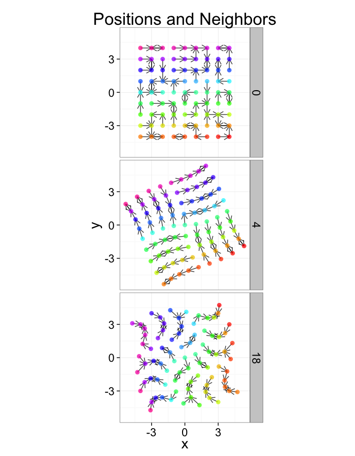
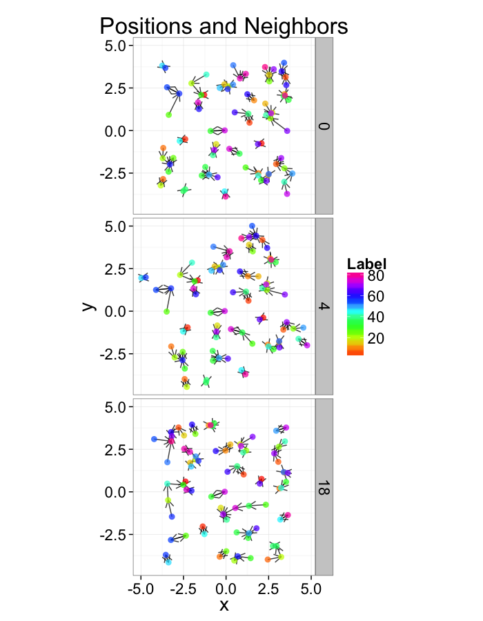
Random Systems
Using a uniform grid of points as a starting point has a strong influence on the results. A better approach is to use a randomly distributed series of points
- resembles real data much better
- avoids these symmetry problems
- \(\epsilon\) sized edges or overlaps
- identical distances to nearby objects
cur.grid<-data.frame(x=runif(81,min=-4,max=4),y=runif(81,min=-4,max=4))
cur.grid$val<-1:nrow(cur.grid)
ggplot(cur.grid,aes(x=x,y=y))+
  geom_point(aes(color=val),size=3,alpha=0.75)+
  labs(title="Positions and Neighbors",color="Label")+
  scale_color_gradientn(colours=rainbow(10))+
    coord_equal()+
  theme_bw(20)
Examining Compression
test.systems.comp<-ldply(c(0.6,1,1.5),function(c.stretch) {
  str.grid<-cur.grid
  str.grid$x<-with(cur.grid,c.stretch*x)
  str.grid$y<-with(cur.grid,c.stretch*y)
  cbind(str.grid,glab=c.stretch)
})

dist.plots.comp<-ddply(test.systems.comp,.(glab),find.nn)
ggplot(test.systems.comp,aes(x=x,y=y))+
  geom_segment(data=dist.plots.comp,aes(xend=xe,yend=ye),
               arrow=arrow(length = unit(0.3,"cm")),alpha=0.75)+
  geom_point(aes(color=val),size=3,alpha=0.75)+
  labs(title="Positions and Neighbors",color="Label")+
  scale_color_gradientn(colours=rainbow(10))+
    coord_equal()+
  facet_grid(glab~.)+
  theme_bw(20)
ggplot(dist.plots.comp,
       aes(x=0,y=0,xend=xe-x,yend=ye-y))+
    geom_density2d(aes(x=xe-x,y=ye-y),color="red",alpha=0.7)+
  geom_segment(aes(color=glab),
               arrow=arrow(length = unit(0.3,"cm")))+
  facet_grid(glab~.)+
    coord_equal()+
  labs(title="Nearest Neighbor Orientations")+guides(color=F)+
  theme_bw(20)
Compression Distributions
ggplot(dist.plots.comp,
       aes(x=dist,fill=as.factor(glab)))+
  geom_histogram(binwidth=0.25)+
  labs(x="NND",title="NN Distances",color="Stretch")+
  scale_y_sqrt()+
  theme_bw(20)
ggplot(dist.plots.comp,
       aes(x=180/pi*atan2(ye-y,xe-x),fill=as.factor(glab)))+
  geom_histogram(binwidth=45)+
    labs(x=expression(paste("NN ",theta)),title="NN Orientation",fill="Stretch")+
  scale_y_sqrt()+
  theme_bw(20)
Examining Different Shears
test.systems.shear<-ldply(c(0,1,3),function(c.shear) {
  str.grid<-cur.grid
  str.grid$x<-with(cur.grid,x+c.shear*(y-2)/2)
  cbind(str.grid,glab=c.shear)
})

dist.plots.shear<-ddply(test.systems.shear,.(glab),find.nn)
ggplot(test.systems.shear,aes(x=x,y=y))+
  geom_segment(data=dist.plots.shear,aes(xend=xe,yend=ye),
               arrow=arrow(length = unit(0.3,"cm")),alpha=0.75)+
  geom_point(aes(color=val),size=3,alpha=0.75)+
  labs(title="Positions and Neighbors",color="Label")+
  scale_color_gradientn(colours=rainbow(10))+
    coord_equal()+
  facet_grid(glab~.)+
  theme_bw(20)
ggplot(dist.plots.shear,
       aes(x=0,y=0,xend=xe-x,yend=ye-y))+
  geom_density2d(aes(x=xe-x,y=ye-y),color="red",alpha=0.7)+
  geom_segment(aes(color=glab),
               arrow=arrow(length = unit(0.3,"cm")))+
  facet_grid(glab~.)+
    coord_equal()+
  labs(title="Nearest Neighbor Orientations")+guides(color=F)+
  theme_bw(20)
Shear Distributions
ggplot(dist.plots.shear,
       aes(x=dist,color=as.factor(glab)))+
  geom_density(size=1.5,adjust=1)+
  labs(x="NND",title="NN Distances",color="Shear")+
  theme_bw(20)
ggplot(dist.plots.shear,
       aes(x=180/pi*atan2(ye-y,xe-x),color=as.factor(glab)))+
  geom_density(size=1.5,adjust=1/1.5)+
    labs(x=expression(paste("NN ",theta)),title="NN Orientation",color="Shear")+
  coord_polar()+
  theme_bw(20)
Examining Different Stretches
str.fun<-function(x,a=1,r=4) sign(x)*r*(abs(x)/r)^a
test.systems<-ldply(c(0.5,1,3),function(c.stretch) {
  str.grid<-cur.grid
  str.grid$x<-with(cur.grid,str.fun(x,a=c.stretch))
  str.grid$y<-with(cur.grid,str.fun(y,a=c.stretch))
  cbind(str.grid,glab=c.stretch)
})

dist.plots<-ddply(test.systems,.(glab),find.nn)
ggplot(test.systems,aes(x=x,y=y))+
  geom_segment(data=dist.plots,aes(xend=xe,yend=ye),
               arrow=arrow(length = unit(0.3,"cm")),alpha=0.75)+
  geom_point(aes(color=val),size=3,alpha=0.75)+
  labs(title="Positions and Neighbors",color="Label")+
  scale_color_gradientn(colours=rainbow(10))+
    coord_equal()+
  facet_grid(glab~.)+
  theme_bw(20)
ggplot(dist.plots,
       aes(x=0,y=0,xend=xe-x,yend=ye-y))+
    geom_density2d(aes(x=xe-x,y=ye-y),color="red",alpha=0.7)+
  geom_segment(aes(color=glab),
               arrow=arrow(length = unit(0.3,"cm")))+
  facet_grid(glab~.)+
    coord_equal()+
  labs(title="Nearest Neighbor Orientations")+guides(color=F)+
  theme_bw(20)
Stretch Distributions
ggplot(dist.plots,
       aes(x=dist,color=as.factor(glab)))+
  geom_density(size=1.5,adjust=1)+
  #geom_histogram(binwidth=0.25)+
  labs(x="NND",title="NN Distances",color="Stretch")+
  theme_bw(20)
ggplot(dist.plots,
       aes(x=180/pi*atan2(ye-y,xe-x),color=as.factor(glab)))+
  #geom_histogram(binwidth=45)+
  geom_density(size=1.5,adjust=1)+
    labs(x=expression(paste("NN ",theta)),title="NN Orientation",color="Stretch")+
  coord_polar()+
  theme_bw(20)
Examining Swirl Systems
cur.grid$cdist<-with(cur.grid,sqrt(x^2+y^2))
test.systems.swirl<-ldply(c(0,pi/40,pi/10),function(c.swirl) {
  str.grid<-cur.grid
  str.grid$x<-with(cur.grid,cos(c.swirl*cdist)*x-sin(c.swirl*cdist)*y)
  str.grid$y<-with(cur.grid,cos(c.swirl*cdist)*y+sin(c.swirl*cdist)*x)
  cbind(str.grid,glab=round(c.swirl*180/pi))
})

dist.plots.swirl<-ddply(test.systems.swirl,.(glab),find.nn)

ggplot(test.systems.swirl,aes(x=x,y=y))+
  geom_segment(data=dist.plots.swirl,aes(xend=xe,yend=ye),
               arrow=arrow(length = unit(0.3,"cm")),alpha=0.75)+
  geom_point(aes(color=val),size=3,alpha=0.75)+
  labs(title="Positions and Neighbors",color="Label")+
  scale_color_gradientn(colours=rainbow(10))+
    coord_equal()+
  facet_grid(glab~.)+
  theme_bw(20)+guides(fill=F)
ggplot(dist.plots.swirl,
       aes(x=0,y=0,xend=xe-x,yend=ye-y))+
    geom_density2d(aes(x=xe-x,y=ye-y),color="red",alpha=0.7)+
  geom_segment(aes(color=glab),
               arrow=arrow(length = unit(0.3,"cm")))+
  facet_grid(glab~.)+
    coord_equal()+
  labs(title="Nearest Neighbor Orientations")+
  theme_bw(20)
Swirl NN Distributions
ggplot(dist.plots.swirl,
       aes(x=dist,color=as.factor(glab)))+
  geom_density()+
  labs(x="NND",title="NN Distances",fill="Swirl")+
  scale_y_sqrt()+
  theme_bw(20)
ggplot(dist.plots.swirl,
       aes(x=180/pi*atan2(ye-y,xe-x),color=as.factor(glab)))+
  geom_density(size=1,adjust=1)+
    labs(x=expression(paste("NN ",theta)),title="NN Orientation",color="Swirl",y="Frequency")+
  #scale_y_sqrt()+
  theme_bw(20)
Voronoi Tesselation
library(deldir)
dd.grid.summary<-function(c.grid,...) {
  c.dd<-deldir(c.grid,...)
  c.vor<-c.dd$dirsgs
  n.pts<-as.vector(summary(as.factor(c(c.vor$ind1,c.vor$ind2))))
  n.vec<-data.frame(ind=1:length(n.pts),
                    n.count=n.pts,
                    area=c.dd$summary$dir.area)
  merge(c.grid,n.vec,by.x="val",by.y="ind")
}
dd.summary<-function(in.df) ddply(in.df,.(glab),dd.grid.summary)
Voronoi tesselation is a method for partitioning a space based on points. The basic idea is that each point \(\vec{p}\) is assigned a region \(\textbf{R}\) consisting of points which are closer to \(\vec{p}\) than any of the other points. Below the diagram is shown in a dashed line for the points shown as small circles.
plot(deldir(std.grid),wlines=c('tess'),showrect=T)
We call the area of a region (\(\textbf{R}\)) around point \(\vec{p}\) its territory.
The grid on the random system, shows much more diversity in territory area.
plot(deldir(cur.grid),wlines=c('tess'),showrect=T)
Calculating Density
Back to our original density problem of having just one number to broadly describe the system.
- Can a voronoi tesselation help us with this?
- YES
With density we calculated
\[ \textrm{Density} = \frac{\textrm{Number of Objects}}{\textrm{Total Volume}} \]
with the regions we have a territory (volume) per object so the average territory is
\[ \bar{Territory} = \frac{\sum \textrm{Territory}_i}{\textrm{Number of Objects}} = \frac{\textrm{Total Volume}}{\textrm{Number of Objects}} = \frac{1}{\textrm{Density}} \]
So the same, but we now have a density definition for a single point!
\[ \textrm{Density}_i = \frac{1}{\textrm{Territory}_i} \]
Density Examples
rand.pnts<-ldply(1:length(dist.funs),function(fun.ind) {
  out.pts<-pt.maker(500,rn.fun=dist.funs[[fun.ind]],fun.ind=fun.ind)
  out.pts$val<-1:nrow(out.pts)
  out.pts
})
ggplot(ddply(rand.pnts,.(fun.ind),function(in.pts) deldir(in.pts)$summary),
       aes(x,y,color=1/dir.area))+
  geom_point()+facet_grid(fun.ind~.)+
  scale_color_gradientn(colours=rainbow(4),trans="log10",limits=c(20,5000))+
  coord_equal()+
  xlim(0,1.01)+ylim(0,1.01)+
  labs(title="Density = 500 N/m^2",color="Local\nDensity")+
  theme_bw(15)
ggplot(cbind(ddply(rand.pnts,.(fun.ind),function(c.block) deldir(c.block,rw=c(0,1,0,1))$summary),mn.pos=500),
       aes(x=1/del.area))+
  geom_density(aes(y=..count..,color="Local"))+
  geom_vline(aes(colour="Average",xintercept=mn.pos))+
  facet_grid(fun.ind~.)+
  scale_x_log10()+
  labs(title="Local Density",x="Density 1/m^2",y="Frequency",color="Density\nMetric")+
  theme_bw(20)
Delaunay Triangulation
A parallel or dual idea where triangles are used and each triangle is created such that the circle which encloses it contains no other points. The triangulation makes the neighbors explicit since connected points in the triangulation correspond to points in our tesselation which share an edge (or face in 3D)
plot(deldir(std.grid),wlines=c('triang'))
We define the number of connections each point \(\vec{p}\) has the Neighbor Count or Delaunay Neighbor Count.
The triangulation on a random system has a much higher diversity in neighbor count
plot(deldir(cur.grid),wlines=c('triang'))
Compression System
Compression
v.comp<-quantile(test.systems.comp$glab,0.2)
plot(deldir(subset(test.systems.comp,glab==v.comp)),wlines=c('tess'),showrect=T)
Tension
v.comp<-quantile(test.systems.comp$glab,0.95)
plot(deldir(subset(test.systems.comp,glab==v.comp)),wlines=c('tess'),showrect=T)
Shear System
Low Shear
v.shear<-min(test.systems.shear$glab)
plot(deldir(subset(test.systems.shear,glab==v.shear)),wlines=c('tess'),showrect=T)
High Shear
v.shear<-max(test.systems.shear$glab)
plot(deldir(subset(test.systems.shear,glab==v.shear)),wlines=c('tess'),showrect=T)
Stretch System
Low Stretch
v.stretch<-min(test.systems$glab)
plot(deldir(subset(test.systems,glab==v.stretch)),wlines=c('tess'),showrect=T)
Highly Stretched System
v.stretch<-quantile(test.systems$glab,0.95)
plot(deldir(subset(test.systems,glab>=v.stretch)),wlines=c('tess'),showrect=T)
Swirl System
Low Swirl System
v.swirl<-min(test.systems.swirl$glab)
plot(deldir(subset(test.systems.swirl,glab==v.swirl)),wlines=c('tess'),showrect=T)
High Swirl System
v.swirl<-max(test.systems.swirl$glab)
plot(deldir(subset(test.systems.swirl,glab==v.swirl)),wlines=c('tess'),showrect=T)
Neighborhoods
Compression
v.comp<-min(test.systems.comp$glab)
plot(deldir(subset(test.systems.comp,glab==v.comp)),wlines=c('triang'),showrect=T)
Stretch
v.stretch<-max(test.systems$glab)
plot(deldir(subset(test.systems,glab==v.stretch)),wlines=c('triang'),showrect=T)
Shear
v.shear<-max(test.systems.shear$glab)
plot(deldir(subset(test.systems.shear,glab==v.shear)),wlines=c('triang'),showrect=T)
Swirl
v.stretch<-quantile(test.systems.swirl$glab,0.95)
plot(deldir(subset(test.systems.swirl,glab==v.stretch)),wlines=c('triang'),showrect=T)
Neighbor Count
test.systems.comp.vor<-dd.summary(test.systems.comp)
test.systems.vor<-dd.summary(test.systems)
test.systems.shear.vor<-dd.summary(test.systems.shear)
test.systems.swirl.vor<-dd.summary(test.systems.swirl)
test.all.vor<-rbind(cbind(test.systems.comp.vor,system="Compression",cdist=0),
      cbind(test.systems.vor,system="Stretching",cdist=0),
      cbind(test.systems.shear.vor,system="Shearing",cdist=0),
      cbind(test.systems.swirl.vor,system="Swirling"))
ggplot(test.all.vor,
       aes(x=n.count))+
  geom_density(aes(color=as.factor(glab)),adjust=1.5)+
  labs(x="Neighbors",color="Stretch")+
  facet_wrap(~system)+
  theme_bw(20)
Volume
ggplot(test.all.vor,
       aes(x=area))+
  geom_density(aes(color=as.factor(glab)))+
  labs(x="Area",color="Stretch")+
  facet_wrap(~system)+
  scale_x_sqrt()+
  theme_bw(20)
Mean vs Variability
ggplot(
  ddply(test.all.vor,.(glab,system),
        function(in.seg) with(in.seg,data.frame(mean.val=mean(n.count),std.val=sd(n.count)))),
  aes(x=as.factor(glab)))+
  geom_line(aes(y=mean.val/20,color="Mean",group=system))+
  geom_line(aes(y=std.val/mean.val,color="Variability",group=system))+
  facet_grid(~system,scales="free_x")+
  labs(x="Parameter",y="Neighbor Count (au)",color="Metric")+
  theme_bw(20)
ggplot(
  ddply(test.all.vor,.(glab,system),
        function(in.seg) with(in.seg,data.frame(mean.val=mean(area),std.val=sd(area)))),
  aes(x=as.factor(glab)))+
  geom_line(aes(y=mean.val/2,color="Mean",group=system))+
  geom_line(aes(y=std.val/mean.val,color="Variability",group=system))+
  facet_grid(~system,scales="free_x")+
  labs(x="Parameter",y="Area (au)",color="Metric")+
  theme_bw(20)
Where are we at?
We have introduced a number of "operations" we can perform on our objects to change their positions
- compression
- stretching
- shearing
- swirling
We have introduced a number of metrics to characterize our images
- Nearest Neighbor distance
- Nearest Neighbor angle
- Delaunay Neigbhor count
- Territory Area (Volume)
A single random systems is useful
- but in order to have a reasonable understanding of the behavior of a system we need to sample many of them.
Understand metrics as a random system + a known transformation
- We take mean values
- Also coefficient of variation (CV) values since they are "scale-free"
m.grid<-function(n.pts=81) {
  out.grid<-data.frame(x=runif(n.pts,min=-4,max=4),y=runif(n.pts,min=-4,max=4))
  out.grid$val<-1:nrow(out.grid)
  out.grid
}
all.metrics<-function(in.grid) {
  nn.df<-find.nn(in.grid)
  vor.df<-dd.grid.summary(in.grid)
  data.frame(NND=mean(nn.df$dist),
             NNTheta=mean(with(nn.df,180/pi*atan2(ye-y,xe-x))),
             DNC=mean(vor.df$n.count),
             Region.Ter=mean(vor.df$area),
             CV.NND=sd(nn.df$dist)/mean(nn.df$dist),
             SD.NNTheta=sd(with(nn.df,180/pi*atan2(ye-y,xe-x))),
             CV.DNC=sd(vor.df$n.count)/mean(vor.df$n.count),
             CV.Region.Ter=sd(vor.df$area)/mean(vor.df$area)
             )
}

many.grid<-function(n.grid,n.pts=81,trans.fun=function(in.pts) in.pts) {
  ldply(1:n.grid,function(n) {
    s.grid<-trans.fun(m.grid(n.pts))
    all.metrics(s.grid)
  },.parallel=T)
}
c.pts<-20
Understanding Metrics
In imaging science we always end up with lots of data, the tricky part is understanding the results that come out.
With this simulation-based approach
- we generate completely random data
- apply a known transformation to it \(\mathcal{F}\)
- quantify the results
We can then take this knowledge and use it to interpret observed data as transformations on an initially random system. We try and find the rules used to produce the sample
Examples
Cell distribution in bone
- Cell position appears random
- Metrics \(\neq\) Random Statistics
- Cells are consistently self-avoiding or stretched
Egg-shell Pores
- Pores in rock / egg shell appear random
- Metrics \(\neq\) Random Statistics
- Pores are also self-avoiding
Compression
comp.sim<-rbind(cbind(many.grid(c.pts),system="No Compression"),
                cbind(many.grid(c.pts,trans.fun=function(in.df) comp.fun(0.75,in.df)),system="Compression"),
                cbind(many.grid(c.pts,trans.fun=function(in.df) comp.fun(1.25,in.df)),system="Tension")
                )
ggplot(melt(comp.sim),aes(x=value,color=system))+
  geom_density()+
  facet_wrap(~variable,scales="free",ncol=4)+
  labs(y="Frequency",x="Value",color="State")+
  theme_bw(20)
Compression Sensitivity
comp.data<-ldply(seq(0.9,1.1,length.out=5),function(c.comp)
  cbind(many.grid(c.pts,trans.fun=function(in.df) comp.fun(c.comp,in.df)),comp=c.comp))


ggplot(melt(comp.data,id.vars=c("comp")),aes(x=comp,y=value))+
  geom_jitter()+
  geom_smooth(method="lm",size=2)+
  labs(y="Value",x="Compression Parameter")+
  facet_wrap(~variable,scale="free_y",ncol=4)+
  theme_bw(20)
Stretching
comp.sim<-rbind(cbind(many.grid(c.pts),system="No Stretch"),
                cbind(many.grid(c.pts,trans.fun=function(in.df) stretch.fun(0.8,in.df)),system="Squeezing"),
                cbind(many.grid(c.pts,trans.fun=function(in.df) stretch.fun(1.2,in.df)),system="Pushing")
                )

ggplot(melt(comp.sim),aes(x=value,color=system))+
  geom_density()+
  facet_wrap(~variable,scales="free",ncol=4)+
  labs(y="Frequency",x="Value",color="State")+
  theme_bw(20)
Stretching Sensitivity
stretch.data<-ldply(seq(0.9,1.1,length.out=5),function(c.stretch)
  cbind(many.grid(c.pts,trans.fun=function(in.df) stretch.fun(c.stretch,in.df)),stretch=c.stretch))

ggplot(melt(stretch.data,id.vars=c("stretch")),aes(x=stretch,y=value))+
  geom_jitter()+
  geom_smooth(method="lm",size=2)+
  labs(y="Value",x="Stretching Parameter")+
  facet_wrap(~variable,scale="free_y",ncol=4)+
  theme_bw(20)
Shearing
comp.sim<-rbind(cbind(many.grid(c.pts),system="No Shear"),
                cbind(many.grid(c.pts,trans.fun=function(in.df) shear.fun(-0.5,in.df)),system="Reverse Shear"),
                cbind(many.grid(c.pts,trans.fun=function(in.df) shear.fun(0.5,in.df)),system="Shear")
                )

ggplot(melt(comp.sim),aes(x=value,color=system))+
  geom_density()+
  facet_wrap(~variable,scales="free",ncol=4)+
  labs(y="Frequency",x="Value",color="State")+
  theme_bw(20)
Shearing Sensitivity
shear.data<-ldply(seq(0,0.2,length.out=5),function(c.shear)
  cbind(many.grid(c.pts,trans.fun=function(in.df) shear.fun(c.shear,in.df)),shear=c.shear))

ggplot(melt(shear.data,id.vars=c("shear")),aes(x=shear,y=value))+
  geom_jitter()+
  geom_smooth(method="lm",size=2)+
  labs(y="Value",x="Shear Parameter")+
  facet_wrap(~variable,scale="free_y",ncol=4)+
  theme_bw(20)
Swirling
comp.sim<-rbind(cbind(many.grid(c.pts),system="No Swirl"),
                cbind(many.grid(c.pts,trans.fun=function(in.df) swirl.fun(0.5,in.df)),system="Some Swirl"),
                cbind(many.grid(c.pts,trans.fun=function(in.df) swirl.fun(2,in.df)),system="Tons of Swirl")
                )

ggplot(melt(comp.sim),aes(x=value,color=system))+
  geom_density()+
  facet_wrap(~variable,scales="free",ncol=4)+
  labs(y="Frequency",x="Value",color="State")+
  theme_bw(20)
Swirling Sensitivity
swirl.data<-ldply(seq(0,0.2,length.out=5),function(c.swirl)
  cbind(many.grid(c.pts,trans.fun=function(in.df) shear.fun(c.swirl,in.df)),swirl=c.swirl))

ggplot(melt(swirl.data,id.vars=c("swirl")),aes(x=swirl,y=value))+
  geom_jitter()+
  geom_smooth(method="lm",size=2)+
  labs(y="Value",x="Swirl Parameter")+
  facet_wrap(~variable,scale="free_y",ncol=4)+
  theme_bw(20)
Self-Avoiding
From the nearest neighbor distance metric, we can create a scale-free version of the metric which we call self-avoiding coefficient or grouping.
The metric is the ratio of
- observed nearest neighbor distance \(\textrm{NND}\)
- the expected mean nearest neighbor distance (\(r_0\)) for a random point distribution (Poisson Point Process) with the same number of points (N.Obj) per volume (Total.Volume).
\[r_0=\sqrt[3]{\frac{\textrm{Total.Volume}}{2\pi \textrm{ N.Obj}}}\]
Using the territory we defined earlier (Region area/volume) we can simplify the definition to
\[ r_0=\sqrt[3]{\frac{\bar{\textrm{Ter}}}{2\pi}} \]
\[ \textrm{SAC} = \frac{\textrm{NND}}{\sqrt[3]{\frac{\bar{\textrm{Ter}}}{2\pi}}} \]
Distribution Tensor
So the information we have is 3D why are we taking single metrics (distance, angle, volume) to quantify it.
- Shouldn't we use 3D metrics with 3D data?
- Just like the shape tensor we covered before, we can define a distribution tensor to characterize the shape of the distribution.
- The major difference instead of constituting voxels we use edges
- an edge is defined from the Delaunay triangluation
- it connects two neighboring bubbles together
- We can calculate distribution for a single bubble by taking all edges that touch the object or from a region by finding all edges inside that region
We start off by calculating the covariance matrix from the list of edges \(\vec{v}_{ij}\) in a given volume \(\mathcal{V}\)
\[ \vec{v}_{ij} = \vec{\textrm{COV}}(i)-\vec{\textrm{COV}}(j) \]
\[ COV(\mathcal{V}) = \frac{1}{N} \sum_{\forall \textrm{COM}(i) \in \mathcal{V}} \begin{bmatrix}
\vec{v}_x\vec{v}_x & \vec{v}_x\vec{v}_y & \vec{v}_x\vec{v}_z\\
\vec{v}_y\vec{v}_x & \vec{v}_y\vec{v}_y & \vec{v}_y\vec{v}_z\\
\vec{v}_z\vec{v}_x & \vec{v}_z\vec{v}_y & \vec{v}_z\vec{v}_z
\end{bmatrix} \]
Distribution Tensor (continued)
We then take the eigentransform of this array to obtain the eigenvectors (principal components, \(\vec{\Lambda}_{1\cdots 3}\)) and eigenvalues (scores, \(\lambda_{1\cdots 3}\))
\[ COV(I_{id}) \longrightarrow \underbrace{\begin{bmatrix}
\vec{\Lambda}_{1x} & \vec{\Lambda}_{1y} & \vec{\Lambda}_{1z} \\
\vec{\Lambda}_{2x} & \vec{\Lambda}_{2y} & \vec{\Lambda}_{2z} \\
\vec{\Lambda}_{3x} & \vec{\Lambda}_{3y} & \vec{\Lambda}_{3z}
\end{bmatrix}}_{\textrm{Eigenvectors}} * \underbrace{\begin{bmatrix}
\lambda_1 & 0 & 0 \\
0 & \lambda_2 & 0 \\
0 & 0 & \lambda_3
\end{bmatrix}}_{\textrm{Eigenvalues}} * \underbrace{\begin{bmatrix}
\vec{\Lambda}_{1x} & \vec{\Lambda}_{1y} & \vec{\Lambda}_{1z} \\
\vec{\Lambda}_{2x} & \vec{\Lambda}_{2y} & \vec{\Lambda}_{2z} \\
\vec{\Lambda}_{3x} & \vec{\Lambda}_{3y} & \vec{\Lambda}_{3z}
\end{bmatrix}^{T}}_{\textrm{Eigenvectors}} \]
The principal components tell us about the orientation of the object and the scores tell us about the corresponding magnitude (or length) in that direction.
Distribution Anisotropy
Visual example
- Tensor represents the average spacing between objects in each direction \(\approx\) thickness of background.
- Its interpretation is more difficult since it doesn't represent a real object
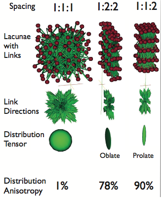
From this tensor we can define an anisotropy in the same manner as we defined for shapes. The anisotropy defined as before
\[ Aiso = \frac{\text{Longest Side}-\text{Shortest Side}}{\text{Longest Side}} \]
- An isotropic distribution tensor indicates the spacing between objects is approximately the same in every direction
- Does not mean a grid, organized, or evenly spaced!
- Just the same in every direction
- Anisotropic distribution tensor means the spacing is smaller in one direction than the others
- Can be regular or grid-like
- Just closer on one direction
Distribution Oblateness
From this tensor we can also define oblateness in the same manner as we defined for shapes. The oblateness is also defined as before as a type of anisotropy
\[ \textrm{Ob} = 2\frac{\lambda_{2}-\lambda_{1}}{\lambda_{3}-\lambda_{1}}-1 \]
- Indicates the pancakeness of the distribution
- Oblate means it is very closely spaced in one direction and far in the other two
- Prolate means it is close in two directions and far in the other
Orientation
The shape tensor provides for each object 3 possible orientations (each of the eigenvectors).
opt.maker<-function(n.pts,rn.fun=function(pts) runif(pts,min=0,max=1),th.amp=0,...) {
  th.val<-runif(n.pts,min=-th.amp,max=th.amp)+pi*round(runif(n.pts))
  data.frame(x=rn.fun(n.pts),y=rn.fun(n.pts),
             xv=cos(th.val),yv=sin(th.val),
             th.amp=th.amp,n.pts=n.pts,
             label=paste("Avg:",round(mean(180/pi*th.val)*10)/10,"Sd:",round(sd(180/pi*th.val)*10)/10),...)
}
or.data<-ldply(seq(1e-1,pi/2.5,length.out=3),function(noise) opt.maker(50,th.amp=noise))

ggplot(or.data,
       aes(x,y,xend=x+0.2*xv,yend=y+0.2*yv))+
  geom_segment(aes(color="Orientation"),arrow=arrow(length = unit(0.15,"cm")))+
  geom_point(aes(color="COV"),alpha=0.7)+
  facet_grid(label~.)+
  coord_equal()+
  labs(color="Type")+
  theme_bw(20)
As we saw in earlier plots it is difficult to express this information in point or graph format
ggplot(or.data,
       aes(x=0,y=0,xend=xv,yend=yv))+
    geom_density2d(aes(x=xv,y=yv),color="red",alpha=0.7)+
  geom_segment(arrow=arrow(length = unit(0.3,"cm")))+
   facet_grid(label~.)+
    coord_equal()+
  labs(title="Object Primary Orientations")+guides(color=F)+
  theme_bw(20)
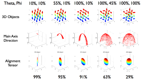
Alignment Tensor
We can again take advantage of the versatility of a tensor representation for our data and use an alignment tensor.
- The same as all of the tensors we have introduced
- Except we use the primary orientation instead of voxel positions (shape) or edges (distribution)
- Similar to distribution it is calculated for a volume (\(\mathcal{V}\)) or region and is meaningless for a single object
\[ \vec{v}_{i} = \vec{\Lambda_1}(i) \]
\[ COV = \frac{1}{N} \sum_{\forall \textrm{COM}(i) \in \mathcal{V}} \begin{bmatrix}
\vec{v}_x\vec{v}_x & \vec{v}_x\vec{v}_y & \vec{v}_x\vec{v}_z\\
\vec{v}_y\vec{v}_x & \vec{v}_y\vec{v}_y & \vec{v}_y\vec{v}_z\\
\vec{v}_z\vec{v}_x & \vec{v}_z\vec{v}_y & \vec{v}_z\vec{v}_z
\end{bmatrix} \]
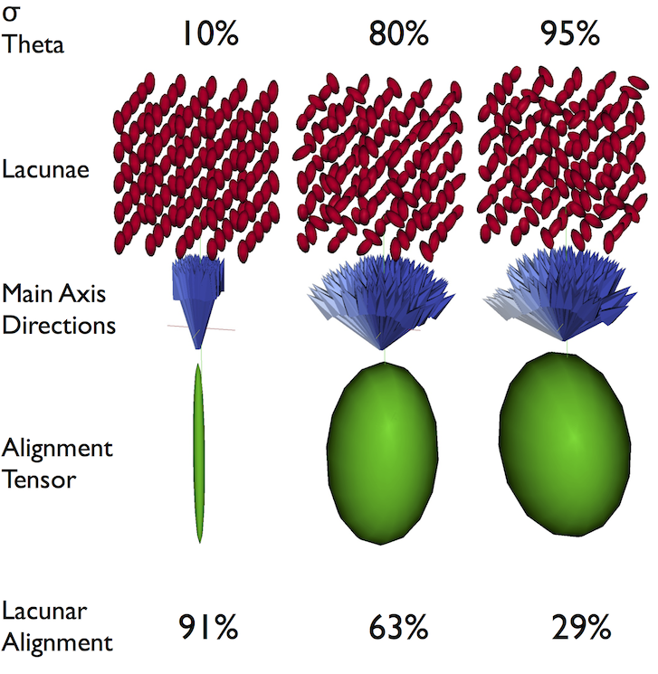
Alignment Anisotropy
Anisotropy for alignment can be summarized as degree of alignment since very anisotropic distributions mean the objects are aligned well in the same direction while an isotropic distribution means the orientations are random. Oblateness can also be defined but is normally not particularly useful.
Other Approaches
K-Means
K-Means can also be used to classify the point-space itself after shape analysis. It is even better suited than for images because while most images are only 2 or 3D the shape vector space can be 50-60 dimensional and is inherently much more difficult to visualize.
2 Point Correlation Functions
For a wider class of analysis of spatial distribution, there exist a class a functions called N-point Correlation Functions