Figure 1.1. TweetDeck provides a highly customizable user interface that can be helpful for analyzing what is happening on Twitter and demonstrates the kind of data that you have access to through the Twitter API
This content is a full-text excerpt from Mining the Social Web (2nd Edition) that has been minimally converted to IPython Notebook format so that you can interactively run the example code as you read the book. The purpose of this offering is to determine if there is sufficient interest to offer the remainder of the entire book as a collection of IPython Notebooks (as a standard distribution format that's in addition to PDF, Kindle, etc.) based on feedback from you.
If you would like to see the full-text of this book (or other books like it) offered in a native IPython Notebook format, tweet something like "@OReillyMedia: Please distribute @SocialWebMining in IPython Notebook format" so that both O'Reilly Media and the author receive your feedback. Alternatively, contact O'Reilly Media using the link above. Thanks!
You can also view this sampler chapter in O'Reilly's new Chimera ebook reader or download a PDF.
This chapter kicks off our journey of mining the social web with Twitter, a rich source of social data that is a great starting point for social web mining because of its inherent openness for public consumption, clean and well-documented API, rich developer tooling, and broad appeal to users from every walk of life. Twitter data is particularly interesting because tweets happen at the "speed of thought" and are available for consumption as they happen in near real time, represent the broadest cross-section of society at an international level, and are so inherently multifaceted. Tweets and Twitter's "following" mechanism link people in a variety of ways, ranging from short (but often meaningful) conversational dialogues to interest graphs that connect people and the things that they care about.
Since this is the first chapter, we'll take our time acclimating to our journey in social web mining. However, given that Twitter data is so accessible and open to public scrutiny, Chapter 9, Twitter Cookbook further elaborates on the broad number of data mining possibilities by providing a terse collection of recipes in a convenient problem/solution format that can be easily manipulated and readily applied to a wide range of problems. You'll also be able to apply concepts from future chapters to Twitter data.
Note:Always get the latest bug-fixed source code for this chapter (and every other chapter) online at http://bit.ly/MiningTheSocialWeb2E. Be sure to also take advantage of this book's virtual machine experience, as described in Appendix A, Information About This Book's Virtual Machine Experience, to maximize your enjoyment of the sample code.
In this chapter, we'll ease into the process of getting situated with a minimal (but effective) development environment with Python, survey Twitter's API, and distill some analytical insights from tweets using frequency analysis. Topics that you'll learn about in this chapter include:
Twitter's developer platform and how to make API requests
Tweet metadata and how to use it
Extracting entities such as user mentions, hashtags, and URLs from tweets
Techniques for performing frequency analysis with Python
Plotting histograms of Twitter data with IPython Notebook
Most chapters won't open with a reflective discussion, but since this is the first chapter of the book and introduces a social website that is often misunderstood, it seems appropriate to take a moment to examine Twitter at a fundamental level.
How would you define Twitter?
There are many ways to answer this question, but let's consider it from an overarching angle that addresses some fundamental aspects of our shared humanity that any technology needs to account for in order to be useful and successful. After all, the purpose of technology is to enhance our human experience.
As humans, what are some things that we want that technology might help us to get?
We want to be heard.
We want to satisfy our curiosity.
We want it easy.
We want it now.
In the context of the current discussion, these are just a few observations that are generally true of humanity. We have a deeply rooted need to share our ideas and experiences, which gives us the ability to connect with other people, to be heard, and to feel a sense of worth and importance. We are curious about the world around us and how to organize and manipulate it, and we use communication to share our observations, ask questions, and engage with other people in meaningful dialogues about our quandaries.
The last two bullet points highlight our inherent intolerance to friction. Ideally, we don't want to have to work any harder than is absolutely necessary to satisfy our curiosity or get any particular job done; we'd rather be doing "something else" or moving on to the next thing because our time on this planet is so precious and short. Along similar lines, we want things now and tend to be impatient when actual progress doesn't happen at the speed of our own thought.
One way to describe Twitter is as a microblogging service that allows people to communicate with short, 140-character messages that roughly correspond to thoughts or ideas. In that regard, you could think of Twitter as being akin to a free, high-speed, global text-messaging service. In other words, it's a glorified piece of valuable infrastructure that enables rapid and easy communication. However, that’s not all of the story. It doesn't adequately address our inherent curiosity and the value proposition that emerges when you have over 500 million curious people registered, with over 100 million of them actively engaging their curiosity on a regular monthly basis.
Besides the macro-level possibilities for marketing and advertising—which are always lucrative with a user base of that size—it's the underlying network dynamics that created the gravity for such a user base to emerge that are truly interesting, and that's why Twitter is all the rage. While the communication bus that enables users to share short quips at the speed of thought may be a necessary condition for viral adoption and sustained engagement on the Twitter platform, it's not a sufficient condition. The extra ingredient that makes it sufficient is that Twitter's asymmetric following model satisfies our curiosity. It is the asymmetric following model that casts Twitter as more of an interest graph than a social network, and the APIs that provide just enough of a framework for structure and self-organizing behavior to emerge from the chaos.
In other words, whereas some social websites like Facebook and LinkedIn require the mutual acceptance of a connection between users (which usually implies a real-world connection of some kind), Twitter's relationship model allows you to keep up with the latest happenings of any other user, even though that other user may not choose to follow you back or even know that you exist. Twitter's following model is simple but exploits a fundamental aspect of what makes us human: our curiosity. Whether it be an infatuation with celebrity gossip, an urge to keep up with a favorite sports team, a keen interest in a particular political topic, or a desire to connect with someone new, Twitter provides you with boundless opportunities to satisfy your curiosity.
Think of an interest graph as a way of modeling connections between people and their arbitrary interests. Interest graphs provide a profound number of possibilities in the data mining realm that primarily involve measuring correlations between things for the objective of making intelligent recommendations and other applications in machine learning. For example, you could use an interest graph to measure correlations and make recommendations ranging from whom to follow on Twitter to what to purchase online to whom you should date. To illustrate the notion of Twitter as an interest graph, consider that a Twitter user need not be a real person; it very well could be a person, but it could also be an inanimate object, a company, a musical group, an imaginary persona, an impersonation of someone (living or dead), or just about anything else.
For example, the @HomerJSimpson account is the official account for Homer Simpson, a popular character from The Simpsons television show. Although Homer Simpson isn't a real person, he's a well-known personality throughout the world, and the @HomerJSimpson Twitter persona acts as an conduit for him (or his creators, actually) to engage his fans. Likewise, although this book will probably never reach the popularity of Homer Simpson, @SocialWebMining is its official Twitter account and provides a means for a community that's interested in its content to connect and engage on various levels. When you realize that Twitter enables you to create, connect, and explore a community of interest for an arbitrary topic of interest, the power of Twitter and the insights you can gain from mining its data become much more obvious.
There is very little governance of what a Twitter account can be aside from the badges on some accounts that identify celebrities and public figures as "verified accounts" and basic restrictions in Twitter's Terms of Service agreement, which is required for using the service. It may seem very subtle, but it's an important distinction from some social websites in which accounts must correspond to real, living people, businesses, or entities of a similar nature that fit into a particular taxonomy. Twitter places no particular restrictions on the persona of an account and relies on self-organizing behavior such as following relationships and folksonomies that emerge from the use of hashtags to create a certain kind of order within the system.
Sidebar Discussion:A fundamental aspect of human intelligence is the desire to classify things and derive a hierarchy in which each element “belongs to” or is a “child” of a parent element one level higher in the hierarchy. Leaving aside some of the finer distinctions between a taxonomy and an ontology, think of a taxonomy as a hierarchical structure like a tree that classifies elements into particular parent/child relationships, whereas a folksonomy (a term coined around 2004) describes the universe of collaborative tagging and social indexing efforts that emerge in various ecosystems of the Web. It’s a play on words in the sense that it blends folk and taxonomy. So, in essence, a folksonomy is just a fancy way of describing the decentralized universe of tags that emerges as a mechanism of collective intelligence when you allow people to classify content with labels. One of the things that's so compelling about the use of hashtags on Twitter is that the folksonomies that organically emerge act as points of aggregation for common interests and provide a focused way to explore while still leaving open the possibility for nearly unbounded serendipity.
Now having a proper frame of reference for Twitter, let us now transition our attention to the problem of acquiring and analyzing Twitter data.
Twitter might be described as a real-time, highly social microblogging service that allows users to post short status updates, called tweets, that appear on timelines. Tweets may include one or more entities in their 140 characters of content and reference one or more places that map to locations in the real world. An understanding of users, tweets, and timelines is particularly essential to effective use of Twitter's API, so a brief introduction to these fundamental Twitter Platform objects is in order before we interact with the API to fetch some data. We've largely discussed Twitter users and Twitter's asymmetric following model for relationships thus far, so this section briefly introduces tweets and timelines in order to round out a general understanding of the Twitter platform.
Tweets are the essence of Twitter, and while they are notionally thought of as the 140 characters of text content associated with a user's status update, there's really quite a bit more metadata there than meets the eye. In addition to the textual content of a tweet itself, tweets come bundled with two additional pieces of metadata that are of particular note: entities and places. Tweet entities are essentially the user mentions, hashtags, URLs, and media that may be associated with a tweet, and places are locations in the real world that may be attached to a tweet. Note that a place may be the actual location in which a tweet was authored, but it might also be a reference to the place described in a tweet.
To make it all a bit more concrete, let's consider a sample tweet with the following text:
@ptwobrussell is writing @SocialWebMining, 2nd Ed. from his home office in Franklin, TN. Be #social: http://on.fb.me/16WJAf9
The tweet is 124 characters long and contains four tweet entities: the user mentions @ptwobrussell and @SocialWebMining, the hashtag #social, and the URL http://on.fb.me/16WJAf9. Although there is a place called Franklin, Tennessee that's explicitly mentioned in the tweet, the places metadata associated with the tweet might include the location in which the tweet was authored, which may or may not be Franklin, Tennessee. That's a lot of metadata that's packed into fewer than 140 characters and illustrates just how potent a short quip can be: it can unambiguously refer to multiple other Twitter users, link to web pages, and cross-reference topics with hashtags that act as points of aggregation and horizontally slice through the entire Twitterverse in an easily searchable fashion.
Finally, timelines are the chronologically sorted collections of tweets. Abstractly, you might say that a timeline is any particular collection of tweets displayed in chronological order; however, you'll commonly see a couple of timelines that are particularly noteworthy. From the perspective of an arbitrary Twitter user, the home timeline is the view that you see when you log into your account and look at all of the tweets from users that you are following, whereas a particular user timeline is a collection of tweets only from a certain user.
For example, when you log into your Twitter account, your home timeline is located at https://twitter.com. The URL for any particular user timeline, however, must be suffixed with a context that identifies the user, such as https://twitter.com/SocialWebMining. If you're interested in seeing what a particular user's home timeline looks like from that user's perspective, you can access it with the additional following suffix appended to the URL. For example, what Tim O'Reilly sees on his home timeline when he logs into Twitter is accessible at https://twitter.com/timoreilly/following.
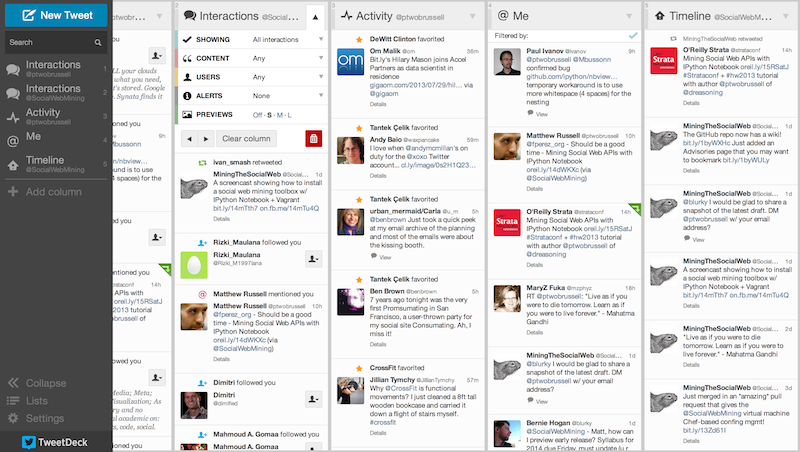
An application like TweetDeck provides several customizable views into the tumultuous landscape of tweets, as shown in Figure 1.1, “TweetDeck provides a highly customizable user interface that can be helpful for analyzing what is happening on Twitter and demonstrates the kind of data that you have access to through the Twitter API”, and is worth trying out if you haven't journeyed far beyond the Twitter.com user interface.
Whereas timelines are collections of tweets with relatively low velocity, streams are samples of public tweets flowing through Twitter in realtime. The public firehose of all tweets has been known to peak at hundreds of thousands of tweets per minute during events with particularly wide interest, such as presidential debates. Twitter's public firehose emits far too much data to consider for the scope of this book and presents interesting engineering challenges, which is at least one of the reasons that various third-party commercial vendors have partnered with Twitter to bring the firehose to the masses in a more consumable fashion. That said, a small random sample of the public timeline is available that provides filterable access to enough public data for API developers to develop powerful applications.
The remainder of this chapter and Part II of this book assume that you have a Twitter account, which is required for API access. If you don't have an account already, take a moment to create onem and then review Twitter’s liberal terms of service, API documentation, and Developer Rules of the Road. The sample code for this chapter and Part II of the book generally don't require you to have any friends or followers of your own, but some of the examples in Part II will be a lot more interesting and fun if you have an active account with a handful of friends and followers that you can use as a basis for social web mining. If you don't have an active account, now would be a good time to get plugged in and start priming your account for the data mining fun to come.
Twitter has taken great care to craft an elegantly simple RESTful API that is intuitive and easy to use. Even so, there are great libraries available to further mitigate the work involved in making API requests. A particularly beautiful Python package that wraps the Twitter API and mimics the public API semantics almost one-to-one is twitter. Like most other Python packages, you can install it with pip by typing pip install twitter in a terminal.
Note:See Appendix C, Python and IPython Notebook Tips & Tricks for instructions on how to install
pip.
Sidebar Discussion:We’ll work though some examples that illustrate the use of the
pydoc) in a few different ways. Outside of a Python shell, runningpydocin your terminal on a package in yourPYTHONPATHis a nice option. For example, on a Linux or Mac system, you can simply typepydoc twitterin a terminal to get the package-level documentation, whereaspydoc twitter.Twitterprovides documentation on thepydocas a package. Typingpython -mpydoc twitter.Twitter, for example, would provide information on thetwitter.Twitterclass. If you find yourself reviewing the documentation for certain modules often, you can elect to pass the-woption topydocand write out an HTML page that you can save and bookmark in your browser.However, more than likely, you'll be in the middle of a working session when you need some help. The built-in
helpfunction accepts a package or class name and is useful for an ordinary Python shell, whereas IPython users can suffix a package or class name with a question mark to view inline help. For example, you could typehelp(twitter)orhelp(twitter.Twitter)in a regular Python interpreter, while you could use the shortcuttwitter?ortwitter.Twitter?in IPython or IPython Notebook.It is highly recommended that you adopt IPython as your standard Python shell when working outside of IPython Notebook because of the various convenience functions, such as tab completion, session history, and "magic functions," that it offers. Recall that Appendix A, Information About This Book's Virtual Machine Experience provides minimal details on getting oriented with recommended developer tools such as IPython.
Note:We'll opt to make programmatic API requests with Python, because the
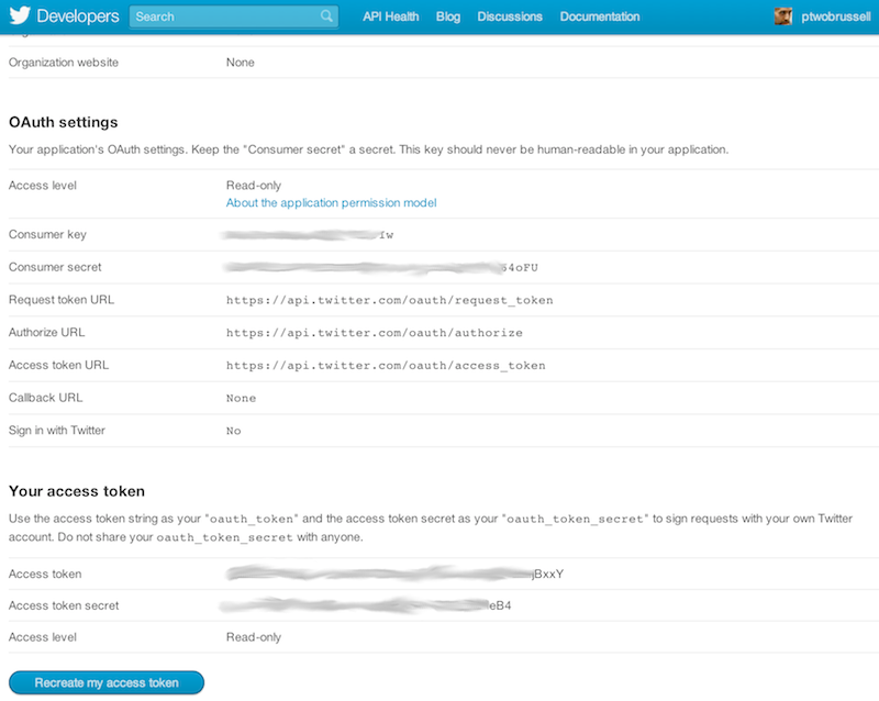
Before you can make any API requests to Twitter, you'll need to create an application at https://dev.twitter.com/apps. Creating an application is the standard way for developers to gain API access and for Twitter to monitor and interact with third-party platform developers as needed. The process for creating an application is pretty standard, and all that's needed is read-only access to the API.
In the present context, you are creating an app that you are going to authorize to access your account data, so this might seem a bit roundabout; why not just plug in your username and password to access the API? While that approach might work fine for you, a third party such as a friend or colleague probably wouldn't feel comfortable forking over a username/password combination in order to enjoy the same insights from your app. Giving up credentials is never a sound practice. Fortunately, some smart people recognized this problem years ago, and now there's a standardized protocol called OAuth (short for Open Authorization) that works for these kinds of situations in a generalized way for the broader social web. The protocol is a social web standard at this point.
If you remember nothing else from this tangent, just remember that OAuth is a means of allowing users to authorize third-party applications to access their account data without needing to share sensitive information like a password. Appendix B, OAuth Primer provides a slightly broader overview of how OAuth works if you're interested, and Twitter's OAuth documentation offers specific details about its particular implementation.[1]
For simplicity of development, the key pieces of information that you'll need to take away from your newly created application's settings are its consumer key, consumer secret, access token, and access token secret. In tandem, these four credentials provide everything that an application would ultimately be getting to authorize itself through a series of redirects involving the user granting authorization, so treat them with the same sensitivity that you would a password.
Note:See Appendix B, OAuth Primer for details on implementing an OAuth 2.0 flow that you would need to build an application that requires an arbitrary user to authorize it to access account data.
Figure 1.2, “Create a new Twitter application to get OAuth credentials and API access at https://dev.twitter.com/apps; the four (blurred) OAuth fields are what you'll use to make API calls to Twitter's API” shows the context of retrieving these credentials.
Without further ado, let’s create an authenticated connection to Twitter's API and find out what people are talking about by inspecting the trends available to us through the GET trends/place resource. While you're at it, go ahead and bookmark the official API documentation as well as the REST API v1.1 resources, because you'll be referencing them regularly as you learn the ropes of the developer-facing side of the Twitterverse.
Note:As of March 2013, Twitter's API operates at version 1.1 and is significantly different in a few areas from the previous v1 API that you may have encountered. Version 1 of the API passed through a deprecation cycle of approximately six months and is no longer operational. All sample code in this book presumes version 1.1 of the API.
Let’s fire up IPython Notebook and initiate a search. Follow along with Example 1.1, “Authorizing an application to access Twitter account data” by substituting your own account credentials into the variables at the beginning of the code example and execute the call to create an instance of the Twitter API. The code works by using your OAuth credentials to create an object called auth that represents your OAuth authorization, which can then be passed to a class called Twitter that is capable of issuing queries to Twitter's API.
import twitter

# XXX: Go to http://dev.twitter.com/apps/new to create an app and get values
# for these credentials, which you'll need to provide in place of these
# empty string values that are defined as placeholders.
# See https://dev.twitter.com/docs/auth/oauth for more information
# on Twitter's OAuth implementation.

CONSUMER_KEY = ''
CONSUMER_SECRET = ''
OAUTH_TOKEN = ''
OAUTH_TOKEN_SECRET = ''

auth = twitter.oauth.OAuth(OAUTH_TOKEN, OAUTH_TOKEN_SECRET,
                           CONSUMER_KEY, CONSUMER_SECRET)

twitter_api = twitter.Twitter(auth=auth)

# Nothing to see by displaying twitter_api except that it's now a
# defined variable

print twitter_api
The results of this example should simply display an unambiguous representation of the twitter_api object that we've constructed, such as:
<twitter.api.Twitter object at 0x39d9b50>
This indicates that we've successfully used OAuth credentials to gain authorization to query Twitter's API.
With an authorized API connection in place, you can now issue a request. Example 1.2, “Retrieving trends” demonstrates how to ask Twitter for the topics that are currently trending worldwide, but keep in mind that the API can easily be parameterized to constrain the topics to more specific locales if you feel inclined to try out some of the possibilities. The device for constraining queries is via Yahoo! GeoPlanet’s Where On Earth (WOE) ID system, which is an API unto itself that aims to provide a way to map a unique identifier to any named place on Earth (or theoretically, even in a virtual world). If you haven't already, go ahead and try out the example that collects a set of trends for both the entire world and just the United States.
# The Yahoo! Where On Earth ID for the entire world is 1.
# See https://dev.twitter.com/docs/api/1.1/get/trends/place and
# http://developer.yahoo.com/geo/geoplanet/

WORLD_WOE_ID = 1
US_WOE_ID = 23424977

# Prefix ID with the underscore for query string parameterization.
# Without the underscore, the twitter package appends the ID value
# to the URL itself as a special case keyword argument.

world_trends = twitter_api.trends.place(_id=WORLD_WOE_ID)
us_trends = twitter_api.trends.place(_id=US_WOE_ID)

print world_trends
print
print us_trends
You should see a semireadable response that is a list of Python dictionaries from the API (as opposed to any kind of error message), such as the following truncated results, before proceeding further. (In just a moment, we'll reformat the response to be more easily readable.)
[{u'created_at': u'2013-03-27T11:50:40Z', u'trends': [{u'url': u'http://twitter.com/search?q=%23MentionSomeoneImportantForYou'...
Notice that the sample result contains a URL for a trend represented as a search query that corresponds to the hashtag #MentionSomeoneImportantForYou, where %23 is the URL encoding for the hashtag symbol. We'll use this rather benign hashtag throughout the remainder of the chapter as a unifying theme for examples that follow. Although a sample data file containing tweets for this hashtag is available with the book's source code, you'll have much more fun exploring a topic that's trending at the time you read this as opposed to following along with a canned topic that is no longer trending.
The pattern for using the twitter module is simple and predictable: instantiate the Twitter class with an object chain corresponding to a base URL and then invoke methods on the object that correspond to URL contexts. For example, twitter_api._trends.place(WORLD_WOE_ID) initiates an HTTP call to GET https://api.twitter.com/1.1/trends/place.json?id=1. Note the URL mapping to the object chain that's constructed with the twitter package to make the request and how query string parameters are passed in as keyword arguments. To use the twitter package for arbitrary API requests, you generally construct the request in that kind of straightforward manner, with just a couple of minor caveats that we'll encounter soon enough.
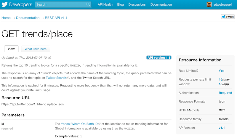
Twitter imposes rate limits on how many requests an application can make to any given API resource within a given time window. Twitter's rate limits are well documented, and each individual API resource also states its particular limits for your convenience. For example, the API request that we just issued for trends limits applications to 15 requests per 15-minute window (see Figure 1.3, “Rate limits for Twitter API resources are identified in the online documentation for each API call; the particular API resource shown here allows 15 requests per "rate limit window," which is currently defined as 15 minutes”). For more nuanced information on how Twitter's rate limits work, see REST API Rate Limiting in v1.1. For the purposes of following along in this chapter, it's highly unlikely that you'll get rate limited. “Making Robust Twitter Requests” (Example 9.16, “Making robust Twitter requests”) will introduce some techniques demonstrating best practices while working with rate limits.
Note:The developer documentation states that the results of a Trends API query are updated only once every five minutes, so it's not a judicious use of your efforts or API requests to ask for results more often than that.
Although it hasn't explicitly been stated yet, the semireadable output from Example 1.2, “Retrieving trends” is printed out as native Python data structures. While an IPython interpreter will "pretty print" the output for you automatically, IPython Notebook and a standard Python interpreter will not. If you find yourself in these circumstances, you may find it handy to use the built-in json package to force a nicer display, as illustrated in Example 1.3, “Displaying API responses as pretty-printed JSON”.
Note:JSON is a data exchange format that you will encounter on a regular basis. In a nutshell, JSON provides a way to arbitrarily store maps, lists, primitives such as numbers and strings, and combinations thereof. In other words, you can theoretically model just about anything with JSON should you desire to do so.
import json

print json.dumps(world_trends, indent=1)
print
print json.dumps(us_trends, indent=1)
An abbreviated sample response from the Trends API produced with json.dumps would look like the following:
[
 {
  "created\_at": "2013-03-27T11:50:40Z",
  "trends": [
   {
    "url": "http://twitter.com/search?q=%23MentionSomeoneImportantForYou",
    "query": "%23MentionSomeoneImportantForYou",
    "name": "\#MentionSomeoneImportantForYou",
    "promoted\_content": null,
    "events": null
   },
   ...
  ]
 }
]
Although it's easy enough to skim the two sets of trends and look for commonality, let's use Python's set data structure to automatically compute this for us, because that's exactly the kind of thing that sets lend themselves to doing. In this instance, a set refers to the mathematical notion of a data structure that stores an unordered collection of unique items and can be computed upon with other sets of items and setwise operations. For example, a setwise intersection computes common items between sets, a setwise union combines all of the items from sets, and the setwise difference among sets acts sort of like a subtraction operation in which items from one set are removed from another.
Example 1.4, “Computing the intersection of two sets of trends” demonstrates how to use a Python list comprehension to parse out the names of the trending topics from the results that were previously queried, cast those lists to sets, and compute the setwise intersection to reveal the common items between them. Keep in mind that there may or may not be significant overlap between any given sets of trends, all depending on what's actually happening when you query for the trends. In other words, the results of your analysis will be entirely dependent upon your query and the data that is returned from it.
Note:Recall that Appendix C, Python and IPython Notebook Tips & Tricks provides a reference for some common Python idioms like list comprehensions that you may find useful to review.
world_trends_set = set([trend['name']
                        for trend in world_trends[0]['trends']])

us_trends_set = set([trend['name']
                     for trend in us_trends[0]['trends']])

common_trends = world_trends_set.intersection(us_trends_set)

print common_trends
Note:You should complete Example 1.4, “Computing the intersection of two sets of trends” before moving on in this chapter to ensure that you are able to access and analyze Twitter data. Can you explain what, if any, correlation exists between trends in your country and the rest of the world?
Sidebar Discussion:Computing setwise operations may seem a rather primitive form of analysis, but the ramifications of set theory for general mathematics are considerably more profound since it provides the foundation for many mathematical principles.
Georg Cantor is generally credited with formalizing the mathematics behind set theory, and his paper “On a Characteristic Property of All Real Algebraic Numbers” (1874) formalized set theory as part of his work on answering questions related to the concept of infinity. To understand how it worked, consider the following question: is the set of positive integers larger in cardinality than the set of both positive and negative integers?
Although common intuition may be that there are twice as many positive and negative integers than positive integers alone, Cantor’s work showed that the cardinalities of the sets are actually equal! Mathematically, he showed that you can map both sets of numbers such that they form a sequence with a definite starting point that extends forever in one direction like this: {1, –1, 2, –2, 3, –3, ...}.
Because the numbers can be clearly enumerated but there is never an ending point, the cardinalities of the sets are said to be countably infinite. In other words, there is a definite sequence that could be followed deterministically if you simply had enough time to count them.
One of the common items between the sets of trending topics turns out to be the hashtag #MentionSomeoneImportantForYou, so let's use it as the basis of a search query to fetch some tweets for further analysis. Example 1.5, “Collecting search results” illustrates how to exercise the GET search/tweets resource for a particular query of interest, including the ability to use a special field that's included in the metadata for the search results to easily make additional requests for more search results. Coverage of Twitter's Streaming API resources is out of scope for this chapter but is introduced in “Sampling the Twitter Firehose with the Streaming API” (Example 9.8, “Sampling the Twitter firehose with the Streaming API”) and may be more appropriate for many situations in which you want to maintain a constantly updated view of tweets.
Note:The use of
*argsand**kwargsas illustrated in Example 1.5, “Collecting search results” as parameters to a function is a Python idiom for expressing arbitrary arguments and keyword arguments, respectively. See Appendix C, Python and IPython Notebook Tips & Tricks for a brief overview of this idiom.
# XXX: Set this variable to a trending topic,
# or anything else for that matter. The example query below
# was a trending topic when this content was being developed
# and is used throughout the remainder of this chapter.

q = '#MentionSomeoneImportantForYou'

count = 100

# See https://dev.twitter.com/docs/api/1.1/get/search/tweets

search_results = twitter_api.search.tweets(q=q, count=count)

statuses = search_results['statuses']


# Iterate through 5 more batches of results by following the cursor

for _ in range(5):
    print "Length of statuses", len(statuses)
    try:
        next_results = search_results['search_metadata']['next_results']
    except KeyError, e: # No more results when next_results doesn't exist
        break

    # Create a dictionary from next_results, which has the following form:
    # ?max_id=313519052523986943&q=NCAA&include_entities=1
    kwargs = dict([ kv.split('=') for kv in next_results[1:].split("&") ])

    search_results = twitter_api.search.tweets(**kwargs)
    statuses += search_results['statuses']

# Show one sample search result by slicing the list...
print json.dumps(statuses[0], indent=1)
Note:Although we're just passing in a hashtag to the Search API at this point, it's well worth noting that it contains a number of powerful operators that allow you to filter queries according to the existence or nonexistence of various keywords, originator of the tweet, location associated with the tweet, etc.
In essence, all the code does is repeatedly make requests to the Search API. One thing that might initially catch you off guard if you've worked with other web APIs (including version 1 of Twitter's API) is that there's no explicit concept of pagination in the Search API itself. Reviewing the API documentation reveals that this is a intentional decision, and there are some good reasons for taking a cursoring approach instead, given the highly dynamic state of Twitter resources. The best practices for cursoring vary a bit throughout the Twitter developer platform, with the Search API providing a slightly simpler way of navigating search results than other resources such as timelines.
Search results contain a special search_metadata node that embeds a next_results field with a query string that provides the basis of a subsequent query. If we weren't using a library like twitter to make the HTTP requests for us, this preconstructed query string would just be appended to the Search API URL, and we'd update it with additional parameters for handling OAuth. However, since we are not making our HTTP requests directly, we must parse the query string into its constituent key/value pairs and provide them as keyword arguments.
In Python parlance, we are unpacking the values in a dictionary into keyword arguments that the function receives. In other words, the function call inside of the for loop in Example 1.5, “Collecting search results” ultimately invokes a function such as twitter_api.search.tweets(q='%23MentionSomeoneImportantForYou', include_entities=1, max_id=313519052523986943) even though it appears in the source code as twitter_api.search.tweets(**kwargs), with kwargs being a dictionary of key/value pairs.
Note:The
search_metadatafield also contains arefresh_urlvalue that can be used if you'd like to maintain and periodically update your collection of results with new information that's become available since the previous query.
The next sample tweet shows the search results for a query for #MentionSomeoneImportantForYou. Take a moment to peruse (all of) it. As I mentioned earlier, there's a lot more to a tweet than meets the eye. The particular tweet that follows is fairly representative and contains in excess of 5 KB of total content when represented in uncompressed JSON. That's more than 40 times the amount of data that makes up the 140 characters of text that's normally thought of as a tweet!
[
 {
  "contributors": null,
  "truncated": false,
  "text": "RT @hassanmusician: \#MentionSomeoneImportantForYou God.",
  "in\_reply\_to\_status\_id": null,
  "id": 316948241264549888,
  "favorite\_count": 0,
  "source": "<a href=\"http://twitter.com/download/android\"...",
  "retweeted": false,
  "coordinates": null,
  "entities": {
   "user\_mentions": [
    {
     "id": 56259379,
     "indices": [
      3,
      18
     ],
     "id\_str": "56259379",
     "screen\_name": "hassanmusician",
     "name": "Download the NEW LP!"
    }
   ],
   "hashtags": [
    {
     "indices": [
      20,
      50
     ],
     "text": "MentionSomeoneImportantForYou"
    }
   ],
   "urls": []
  },
  "in\_reply\_to\_screen\_name": null,
  "in\_reply\_to\_user\_id": null,
  "retweet\_count": 23,
  "id\_str": "316948241264549888",
  "favorited": false,
  "retweeted\_status": {
   "contributors": null,
   "truncated": false,
   "text": "\#MentionSomeoneImportantForYou God.",
   "in\_reply\_to\_status\_id": null,
   "id": 316944833233186816,
   "favorite\_count": 0,
   "source": "web",
   "retweeted": false,
   "coordinates": null,
   "entities": {
    "user\_mentions": [],
    "hashtags": [
     {
      "indices": [
       0,
       30
      ],
      "text": "MentionSomeoneImportantForYou"
     }
    ],
    "urls": []
   },
   "in\_reply\_to\_screen\_name": null,
   "in\_reply\_to\_user\_id": null,
   "retweet\_count": 23,
   "id\_str": "316944833233186816",
   "favorited": false,
   "user": {
    "follow\_request\_sent": null,
    "profile\_use\_background\_image": true,
    "default\_profile\_image": false,
    "id": 56259379,
    "verified": false,
    "profile\_text\_color": "3C3940",
    "profile\_image\_url\_https": "https://si0.t...",
    "profile\_sidebar\_fill\_color": "95E8EC",
    "entities": {
     "url": {
      "urls": [
       {
        "url": "http://t.co/yRX89YM4J0",
        "indices": [
         0,
         22
        ],
        "expanded\_url": "http://www.datpiff...",
        "display\_url": "datpiff.com/mixtapes-detai\u2026"
       }
      ]
     },
     "description": {
      "urls": []
     }
    },
    "followers\_count": 105041,
    "profile\_sidebar\_border\_color": "000000",
    "id\_str": "56259379",
    "profile\_background\_color": "000000",
    "listed\_count": 64,
    "profile\_background\_image\_url\_https": "https://si0.t...",
    "utc\_offset": -18000,
    "statuses\_count": 16691,
    "description": "\#TheseAreTheWordsISaid LP",
    "friends\_count": 59615,
    "location": "",
    "profile\_link\_color": "91785A",
    "profile\_image\_url": "http://a0.twimg.com/...",
    "following": null,
    "geo\_enabled": true,
    "profile\_banner\_url": "https://si0.twimg.com/pr...",
    "profile\_background\_image\_url": "http://a0.twi...",
    "screen\_name": "hassanmusician",
    "lang": "en",
    "profile\_background\_tile": false,
    "favourites\_count": 6142,
    "name": "Download the NEW LP!",
    "notifications": null,
    "url": "http://t.co/yRX89YM4J0",
    "created\_at": "Mon Jul 13 02:18:25 +0000 2009",
    "contributors\_enabled": false,
    "time\_zone": "Eastern Time (US & Canada)",
    "protected": false,
    "default\_profile": false,
    "is\_translator": false
   },
   "geo": null,
   "in\_reply\_to\_user\_id\_str": null,
   "lang": "en",
   "created\_at": "Wed Mar 27 16:08:31 +0000 2013",
   "in\_reply\_to\_status\_id\_str": null,
   "place": null,
   "metadata": {
    "iso\_language\_code": "en",
    "result\_type": "recent"
   }
  },
  "user": {
   "follow\_request\_sent": null,
   "profile\_use\_background\_image": true,
   "default\_profile\_image": false,
   "id": 549413966,
   "verified": false,
   "profile\_text\_color": "3D1957",
   "profile\_image\_url\_https": "https://si0.twimg...",
   "profile\_sidebar\_fill\_color": "7AC3EE",
   "entities": {
    "description": {
     "urls": []
    }
   },
   "followers\_count": 110,
   "profile\_sidebar\_border\_color": "FFFFFF",
   "id\_str": "549413966",
   "profile\_background\_color": "642D8B",
   "listed\_count": 1,
   "profile\_background\_image\_url\_https": "https:...",
   "utc\_offset": 0,
   "statuses\_count": 1294,
   "description": "i BELIEVE do you? I admire n adore @justinbieber ",
   "friends\_count": 346,
   "location": "All Around The World ",
   "profile\_link\_color": "FF0000",
   "profile\_image\_url": "http://a0.twimg.com/pr...",
   "following": null,
   "geo\_enabled": true,
   "profile\_banner\_url": "https://si0.twimg.com/...",
   "profile\_background\_image\_url": "http://a0.tw...",
   "screen\_name": "LilSalima",
   "lang": "en",
   "profile\_background\_tile": true,
   "favourites\_count": 229,
   "name": "KoKo :D",
   "notifications": null,
   "url": null,
   "created\_at": "Mon Apr 09 17:51:36 +0000 2012",
   "contributors\_enabled": false,
   "time\_zone": "London",
   "protected": false,
   "default\_profile": false,
   "is\_translator": false
  },
  "geo": null,
  "in\_reply\_to\_user\_id\_str": null,
  "lang": "en",
  "created\_at": "Wed Mar 27 16:22:03 +0000 2013",
  "in\_reply\_to\_status\_id\_str": null,
  "place": null,
  "metadata": {
   "iso\_language\_code": "en",
   "result\_type": "recent"
  }
 },
 ...
]
Tweets are imbued with some of the richest metadata that you'll find on the social web, and Chapter 9, Twitter Cookbook elaborates on some of the many possibilities.
The online documentation is always the definitive source for Twitter platform objects, and it's worthwhile to bookmark the Tweets page, because it's one that you'll refer to quite frequently as you get familiarized with the basic anatomy of a tweet. No attempt is made here or elsewhere in the book to regurgitate online documentation, but a few notes are of interest given that you might still be a bit overwhelmed by the 5 KB of information that a tweet comprises. For simplicity of nomenclature, let's assume that we've extracted a single tweet from the search results and stored it in a variable named t. For example, t.keys() returns the top-level fields for the tweet and t['id'] accesses the identifier of the tweet.
Note:If you're following along with the IPython Notebook for this chapter, the exact tweet that's under scrutiny is stored in a variable named
tso that you can interactively access its fields and explore more easily. The current discussion assumes the same nomenclature, so values should correspond one-for-one.
The human-readable text of a tweet is available through t['text']:
The entities in the text of a tweet are conveniently processed for you and available through t['entities']:
Clues as to the "interestingness" of a tweet are available through t['favorite_count'] and t['retweet_count'], which return the number of times it's been bookmarked or retweeted, respectively.
If a tweet has been retweeted, the t['retweeted_status'] field provides significant detail about the original tweet itself and its author. Keep in mind that sometimes the text of a tweet changes as it is retweeted, as users add reactions or otherwise manipulate the text.
The t['retweeted'] field denotes whether or not the authenticated user (via an authorized application) has retweeted this particular tweet. Fields that vary depending upon the point of view of the particular user are denoted in Twitter's developer documentation as perspectival, which means that their values will vary depending upon the perspective of the user.
Additionally, note that only original tweets are retweeted from the standpoint of the API and information management. Thus, the retweet_count reflects the total number of times that the original tweet has been retweeted and should reflect the same value in both the original tweet and all subsequent retweets. In other words, retweets aren't retweeted. It may be a bit counterintuitive at first, but if you think you're retweeting a retweet, you're actually just retweeting the original tweet that you were exposed to through a proxy. See “Examining Patterns in Retweets” later in this chapter for a more nuanced discussion about the difference between retweeting vs quoting a tweet.
You should tinker around with the sample tweet and consult the documentation to clarify any lingering questions you might have before moving forward. A good working knowledge of a tweet's anatomy is critical to effectively mining Twitter data.
Next, let's distill the entities and the text of the tweets into a convenient data structure for further examination. Example 1.6, “Extracting text, screen names, and hashtags from tweets” extracts the text, screen names, and hashtags from the tweets that are collected and introduces a Python idiom called a double (or nested) list comprehension. If you understand a (single) list comprehension, the code formatting should illustrate the double list comprehension as simply a collection of values that are derived from a nested loop as opposed to the results of a single loop. List comprehensions are particularly powerful because they usually yield substantial performance gains over nested lists and provide an intuitive (once you’re familiar with them) yet terse syntax.
Note:List comprehensions are used frequently throughout this book, and it's worth consulting Appendix C, Python and IPython Notebook Tips & Tricks or the official Python tutorial for more details if you'd like additional context.
status_texts = [ status['text']
                 for status in statuses ]

screen_names = [ user_mention['screen_name']
                 for status in statuses
                     for user_mention in status['entities']['user_mentions'] ]

hashtags = [ hashtag['text']
             for status in statuses
                 for hashtag in status['entities']['hashtags'] ]

# Compute a collection of all words from all tweets
words = [ w
          for t in status_texts
              for w in t.split() ]

# Explore the first 5 items for each...

print json.dumps(status_texts[0:5], indent=1)
print json.dumps(screen_names[0:5], indent=1)
print json.dumps(hashtags[0:5], indent=1)
print json.dumps(words[0:5], indent=1)
Sample output follows; it displays five status texts, screen names, and hashtags to provide a feel for what's in the data.
Note:In Python, syntax in which square brackets appear after a list or string value, such as
status_texts[0:5], is indicative of slicing, whereby you can easily extract items from lists or substrings from strings. In this particular case,[0:5]indicates that you'd like the first five items in the liststatus_texts(corresponding to items at indices 0 through 4). See Appendix C, Python and IPython Notebook Tips & Tricks for a more extended description of slicing in Python.
[ "201c@KathleenMariee_: #MentionSomeOneImportantForYou @AhhlicksCruise..., "#MentionSomeoneImportantForYou My bf @Linkin_Sunrise.", "RT @hassanmusician: #MentionSomeoneImportantForYou God.", "#MentionSomeoneImportantForYou @Louis_Tomlinson", "#MentionSomeoneImportantForYou @Delta_Universe" ] [ "KathleenMariee_", "AhhlicksCruise", "itsravennn_cx", "kandykisses_13", "BMOLOGY" ] [ "MentionSomeOneImportantForYou", "MentionSomeoneImportantForYou", "MentionSomeoneImportantForYou", "MentionSomeoneImportantForYou", "MentionSomeoneImportantForYou" ] [ "201c@KathleenMariee_:", "#MentionSomeOneImportantForYou", "@AhhlicksCruise", ",", "@itsravennn_cx" ]
As expected, #MentionSomeoneImportantForYou dominates the hashtag output. The output also provides a few commonly occurring screen names that are worth investigating.
Virtually all analysis boils down to the simple exercise of counting things on some level, and much of what we'll be doing in this book is manipulating data so that it can be counted and further manipulated in meaningful ways.
From an empirical standpoint, counting observable things is the starting point for just about everything, and thus the starting point for any kind of statistical filtering or manipulation that strives to find what may be a faint signal in noisy data. Whereas we just extracted the first 5 items of each unranked list to get a feel for the data, let's now take a closer look at what's in the data by computing a frequency distribution and looking at the top 10 items in each list.
As of Python 2.7, a collections module is available that provides a counter that makes computing a frequency distribution rather trivial. Example 1.7, “Creating a basic frequency distribution from the words in tweets” demonstrates how to use a Counter to compute frequency distributions as ranked lists of terms. Among the more compelling reasons for mining Twitter data is to try to answer the question of what people are talking about right now. One of the simplest techniques you could apply to answer this question is basic frequency analysis, just as we are performing here.
from collections import Counter

for item in [words, screen_names, hashtags]:
    c = Counter(item)
    print c.most_common()[:10] # top 10
    print
Here are some sample results from frequency analysis of tweets:
[(u'\#MentionSomeoneImportantForYou', 92), (u'RT', 34), (u'my', 10),
 (u',', 6), (u'@justinbieber', 6), (u'<3', 6), (u'My', 5), (u'and', 4),
 (u'I', 4), (u'te', 3)]

[(u'justinbieber', 6), (u'Kid\_Charliej', 2), (u'Cavillafuerte', 2),
 (u'touchmestyles\_', 1), (u'aliceorr96', 1), (u'gymleeam', 1), (u'fienas', 1),
 (u'nayely\_1D', 1), (u'angelchute', 1)]

[(u'MentionSomeoneImportantForYou', 94), (u'mentionsomeoneimportantforyou', 3),
 (u'NoHomo', 1), (u'Love', 1), (u'MentionSomeOneImportantForYou', 1),
 (u'MyHeart', 1),  (u'bebesito', 1)]
The result of the frequency distribution is a map of key/value pairs corresponding to terms and their frequencies, so let's make reviewing the results a little easier on the eyes by emitting a tabular format. You can install a package called prettytable by typing pip install prettytable in a terminal; this package provides a convenient way to emit a fixed-width tabular format that can be easily copied-and-pasted.
Example 1.8, “Using prettytable to display tuples in a nice tabular format” shows how to use it to display the same results.
from prettytable import PrettyTable

for label, data in (('Word', words),
                    ('Screen Name', screen_names),
                    ('Hashtag', hashtags)):
    pt = PrettyTable(field_names=[label, 'Count'])
    c = Counter(data)
    [ pt.add_row(kv) for kv in c.most_common()[:10] ]
    pt.align[label], pt.align['Count'] = 'l', 'r' # Set column alignment
    print pt
The results from Example 1.8, “Using prettytable to display tuples in a nice tabular format” are displayed as a series of nicely formatted text-based tables that are easy to skim, as the following output demonstrates.
+--------------------------------+-------+
| Word                           | Count |
+--------------------------------+-------+
| \#MentionSomeoneImportantForYou |    92 |
| RT                             |    34 |
| my                             |    10 |
| ,                              |     6 |
| @justinbieber                  |     6 |
| <3                          |     6 |
| My                             |     5 |
| and                            |     4 |
| I                              |     4 |
| te                             |     3 |
+--------------------------------+-------+
+----------------+-------+
| Screen Name    | Count |
+----------------+-------+
| justinbieber   |     6 |
| Kid\_Charliej   |     2 |
| Cavillafuerte  |     2 |
| touchmestyles\_ |     1 |
| aliceorr96     |     1 |
| gymleeam       |     1 |
| fienas         |     1 |
| nayely\_1D      |     1 |
| angelchute     |     1 |
+----------------+-------+
+-------------------------------+-------+
| Hashtag                       | Count |
+-------------------------------+-------+
| MentionSomeoneImportantForYou |    94 |
| mentionsomeoneimportantforyou |     3 |
| NoHomo                        |     1 |
| Love                          |     1 |
| MentionSomeOneImportantForYou |     1 |
| MyHeart                       |     1 |
| bebesito                      |     1 |
+-------------------------------+-------+
A quick skim of the results reveals at least one marginally surprising thing: Justin Bieber is high on the list of entities for this small sample of data, and given his popularity with tweens on Twitter he may very well have been the "most important someone" for this trending topic, though the results here are inconclusive. The appearance of <3 is also interesting because it is an escaped form of <3, which represents a heart shape (that's rotated 90 degrees, like other emoticons and smileys) and is a common abbreviation for "loves." Given the nature of the query, it's not surprising to see a value like <3, although it may initially seem like junk or noise.
Although the entities with a frequency greater than two are interesting, the broader results are also revealing in other ways. For example, "RT" was a very common token, implying that there were a significant number of retweets (we'll investigate this observation further in “Examining Patterns in Retweets”). Finally, as might be expected, the #MentionSomeoneImportantForYou hashtag and a couple of case-sensitive variations dominated the hashtags; a data-processing takeaway is that it would be worthwhile to normalize each word, screen name, and hashtag to lowercase when tabulating frequencies since there will inevitably be variation in tweets.
A slightly more advanced measurement that involves calculating simple frequencies and can be applied to unstructured text is a metric called lexical diversity. Mathematically, this is an expression of the number of unique tokens in the text divided by the total number of tokens in the text, which are both elementary yet important metrics in and of themselves. Lexical diversity is an interesting concept in the area of interpersonal communications because it provides a quantitative measure for the diversity of an individual's or group's vocabulary. For example, suppose you are listening to someone who repeatedly says "and stuff" to broadly generalize information as opposed to providing specific examples to reinforce points with more detail or clarity. Now, contrast that speaker to someone else who seldom uses the word "stuff" to generalize and instead reinforces points with concrete examples. The speaker who repeatedly says "and stuff" would have a lower lexical diversity than the speaker who uses a more diverse vocabulary, and chances are reasonably good that you'd walk away from the conversation feeling as though the speaker with the higher lexical diversity understands the subject matter better.
As applied to tweets or similar online communications, lexical diversity can be worth considering as a primitive statistic for answering a number of questions, such as how broad or narrow the subject matter is that an individual or group discusses. Although an overall assessment could be interesting, breaking down the analysis to specific time periods could yield additional insight, as could comparing different groups or individuals. For example, it would be interesting to measure whether or not there is a significant difference between the lexical diversity of two soft drink companies such as Coca-Cola and Pepsi as an entry point for exploration if you were comparing the effectiveness of their social media marketing campaigns on Twitter.
With a basic understanding of how to use a statistic like lexical diversity to analyze textual content such as tweets, let's now compute the lexical diversity for statuses, screen names, and hashtags for our working data set, as shown in Example 1.9, “Calculating lexical diversity for tweets”.
# A function for computing lexical diversity
def lexical_diversity(tokens):
    return 1.0*len(set(tokens))/len(tokens)

# A function for computing the average number of words per tweet
def average_words(statuses):
    total_words = sum([ len(s.split()) for s in statuses ])
    return 1.0*total_words/len(statuses)

print lexical_diversity(words)
print lexical_diversity(screen_names)
print lexical_diversity(hashtags)
print average_words(status_texts)
The results of Example 1.9, “Calculating lexical diversity for tweets” follow:
0.67610619469
0.955414012739
0.0686274509804
5.76530612245
There are a few observations worth considering in the results:
The lexical diversity of the words in the text of the tweets is around 0.67. One way to interpret that figure would be to say that about two out of every three words is unique, or you might say that each status update carries around 67% unique information. Given that the average number of words in each tweet is around six, that translates to about four unique words per tweet. Intuition aligns with the data in that the nature of a #MentionSomeoneImportantForYou trending hashtag is to solicit a response that will probably be a few words long. In any event, a value of 0.67 is on the high side for lexical diversity of ordinary human communication, but given the nature of the data, it seems very reasonable.
The lexical diversity of the screen names, however, is even higher, with a value of 0.95, which means that about 19 out of 20 screen names mentioned are unique. This observation also makes sense given that many answers to the question will be a screen name, and that most people won't be providing the same responses for the solicitous hashtag.
The lexical diversity of the hashtags is extremely low at a value of around 0.068, implying that very few values other than the #MentionSomeoneImportantForYou hashtag appear multiple times in the results. Again, this makes good sense given that most responses are short and that hashtags really wouldn't make much sense to introduce as a response to the prompt of mentioning someone important for you.
The average number of words per tweet is very low at a value of just under 6, which makes sense given the nature of the hashtag, which is designed to solicit short responses consisting of just a few words.
What would be interesting at this point would be to zoom in on some of the data and see if there were any common responses or other insights that could come from a more qualitative analysis. Given an average number of words per tweet as low as 6, it's unlikely that users applied any abbreviations to stay within the 140 characters, so the amount of noise for the data should be remarkably low, and additional frequency analysis may reveal some fascinating things.
Even though the user interface and many Twitter clients have long since adopted the native Retweet API used to populate status values such as retweet_count and retweeted_status, some Twitter users may prefer to quote a tweet, which entails a workflow involving copying and pasting the text and prepending "RT @username" or suffixing "/via @username" to provide attribution.
Note:When mining Twitter data, you'll probably want to both account for the tweet metadata and use heuristics to analyze the 140 characters for conventions such as "RT @username" or "/via @username" when considering retweets, in order to maximize the efficacy of your analysis. See “Finding Users Who Have Retweeted a Status” for a more detailed discussion on retweeting with Twitter's native Retweet API versus "quoting" tweets and using conventions to apply attribution.
A good exercise at this point would be to further analyze the data to determine if there was a particular tweet that was highly retweeted or if there were just lots of "one-off" retweets. The approach we'll take to find the most popular retweets is to simply iterate over each status update and store out the retweet count, originator of the retweet, and text of the retweet if the status update is a retweet. Example 1.10, “Finding the most popular retweets” demonstrates how to capture these values with a list comprehension and sort by the retweet count to display the top few results.
retweets = [
            # Store out a tuple of these three values ...
            (status['retweet_count'],
             status['retweeted_status']['user']['screen_name'],
             status['text'])

            # ... for each status ...
            for status in statuses

            # ... so long as the status meets this condition.
                if status.has_key('retweeted_status')
           ]

# Slice off the first 5 from the sorted results and display each item in the tuple

pt = PrettyTable(field_names=['Count', 'Screen Name', 'Text'])
[ pt.add_row(row) for row in sorted(retweets, reverse=True)[:5] ]
pt.max_width['Text'] = 50
pt.align= 'l'
print pt
Results from Example 1.10, “Finding the most popular retweets” are interesting:
+-------+----------------+----------------------------------------------------+
| Count | Screen Name    | Text                                               |
+-------+----------------+----------------------------------------------------+
| 23    | hassanmusician | RT @hassanmusician: \#MentionSomeoneImportantForYou |
|       |                | God.                                               |
| 21    | HSweethearts   | RT @HSweethearts: \#MentionSomeoneImportantForYou   |
|       |                | my high school sweetheart ❤                        |
| 15    | LosAlejandro\_  | RT @LosAlejandro\_: ¿Nadie te menciono en           |
|       |                | "\#MentionSomeoneImportantForYou"? JAJAJAJAJAJAJAJA |
|       |                | JAJAJAJAJAJAJAJAJAJAJAJAJAJAJAJAJAJAJAJA Ven, ...  |
| 9     | SCOTTSUMME     | RT @SCOTTSUMME: \#MentionSomeoneImportantForYou My  |
|       |                | Mum. Shes loving, caring, strong, all in one. I    |
|       |                | love her so much ❤❤❤❤                            |
| 7     | degrassihaha   | RT @degrassihaha: \#MentionSomeoneImportantForYou I |
|       |                | can't put every Degrassi cast member, crew member, |
|       |                | and writer in just one tweet....                   |
+-------+----------------+----------------------------------------------------+
"God" tops the list, followed closely by "my high school sweetheart," and coming in at number four on the list is "My Mum." None of the top five items in the list correspond to Twitter user accounts, although we might have suspected this (with the exception of @justinbieber) from the previous analysis. Inspection of results further down the list does reveal particular user mentions, but the sample we have drawn from for this query is so small that no trends emerge. Searching for a larger sample of results would likely yield some user mentions with a frequency greater than one, which would be interesting to further analyze. The possibilities for further analysis are pretty open-ended, and by now, hopefully, you're itching to try out some custom queries of your own.
Note:Suggested exercises are at the end of this chapter. Be sure to also check out Chapter 9, Twitter Cookbook as a source of inspiration: it includes more than two dozen recipes presented in a cookbook-style format.
Before we move on, a subtlety worth noting is that it's quite possible (and probable, given the relatively low frequencies of the retweets observed in this section) that the original tweets that were retweeted may not exist in our sample search results set. For example, the most popular retweet in the sample results originated from a user with a screen name of @hassanmusician and was retweeted 23 times. However, closer inspection of the data reveals that we collected only 1 of the 23 retweets in our search results. Neither the original tweet nor any of the other 22 retweets appears in the data set. This doesn't pose any particular problems, although it might beg the question of who the other 22 retweeters for this status were.
The answer to this kind of question is a valuable one because it allows us to take content that represents a concept, such as "God" in this case, and discover a group of other users who apparently share the same sentiment or common interest. As previously mentioned, a handy way to model data involving people and the things that they're interested in is called an interest graph; this is the primary data structure that supports analysis in Chapter 7, Mining GitHub: Inspecting Software Collaboration Habits, Building Interest Graphs, and More. Interpretative speculation about these users could suggest that they are spiritual or religious individuals, and further analysis of their particular tweets might corroborate that inference. Example 1.11, “Looking up users who have retweeted a status” shows how to find these individuals with the GET statuses/retweets/:id API.
# Get the original tweet id for a tweet from its retweeted_status node
# and insert it here in place of the sample value that is provided
# from the text of the book

_retweets = twitter_api.statuses.retweets(id=317127304981667841)
print [r['user']['screen_name'] for r in _retweets]
Further analysis of the users who retweeted this particular status for any particular religious or spiritual affiliation is left as an independent exercise.
A nice feature of IPython Notebook is its ability to generate and insert high-quality and customizable plots of data as part of an interactive workflow. In particular, the matplotlib package and other scientific computing tools that are available for IPython Notebook are quite powerful and capable of generating complex figures with very little effort once you understand the basic workflows.
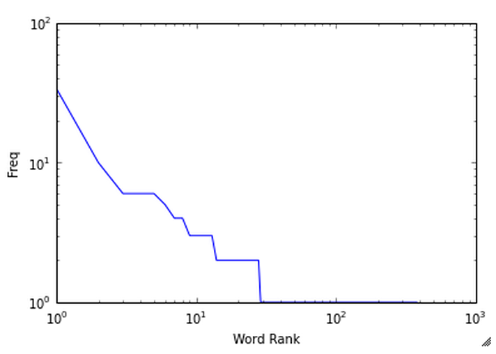
To illustrate the use of matplotlib's plotting capabilities, let's plot some data for display. To get warmed up, we’ll consider a plot that displays the results from the words variable as defined in Example 1.9, “Calculating lexical diversity for tweets”. With the help of a Counter, it's easy to generate a sorted list of tuples where each tuple is a (word, frequency) pair; the x-axis value will correspond to the index of the tuple, and the y-axis will correspond to the frequency for the word in that tuple. It would generally be impractical to try to plot each word as a value on the x-axis, although that's what the x-axis is representing. Figure 1.4, “A plot displaying the sorted frequencies for the words computed by Example 1.8, “Using prettytable to display tuples in a nice tabular format”” displays a plot for the same words data that we previously rendered as a table in Example 1.8, “Using prettytable to display tuples in a nice tabular format”. The y-axis values on the plot correspond to the number of times a word appeared. Although labels for each word are not provided, x-axis values have been sorted so that the relationship between word frequencies is more apparent. Each axis has been adjusted to a logarithmic scale to "squash" the curve being displayed. The plot can be generated directly in IPython Notebook with the code shown in Example 1.12, “Plotting frequencies of words”.
Note:If you are using the virtual machine, your IPython Notebooks should be configured to use plotting capabilities out of the box. If you are running on your own local environment, be sure to have started IPython Notebook with PyLab enabled as follows:
ipython notebook --pylab=inline
word_counts = sorted(Counter(words).values(), reverse=True)

plt.loglog(word_counts)
plt.ylabel("Freq")
plt.xlabel("Word Rank")
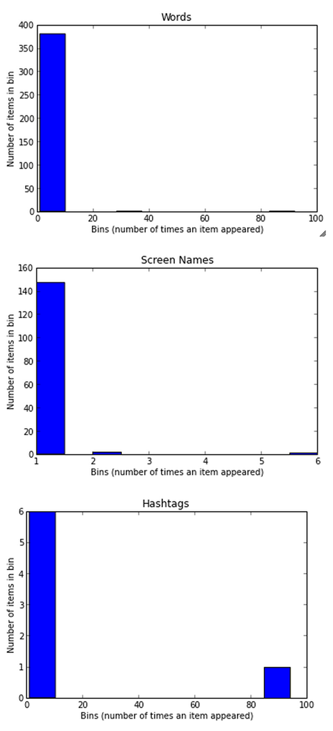
A plot of frequency values is intuitive and convenient, but it can also be useful to group together data values into bins that correspond to a range of frequencies. For example, how many words have a frequency between 1 and 5, between 5 and 10, between 10 and 15, and so forth? A histogram is designed for precisely this purpose and provides a convenient visualization for displaying tabulated frequencies as adjacent rectangles, where the area of each rectangle is a measure of the data values that fall within that particular range of values. Figures 1.5 and 1.6 show histograms of the tabular data generated from Examples 1.8 and 1.10, respectively. Although the histograms don't have x-axis labels that show us which words have which frequencies, that's not really their purpose. A histogram gives us insight into the underlying frequency distribution, with the x-axis corresponding to a range for words that each have a frequency within that range and the y-axis corresponding to the total frequency of all words that appear within that range.
When interpreting Figure 1.5, “Histograms of tabulated frequency data for words, screen names, and hashtags, each displaying a particular kind of data that is grouped by frequency”, look back to the corresponding tabular data and consider that there are a large number of words, screen names, or hashtags that have low frequencies and appear few times in the text; however, when we combine all of these low-frequency terms and bin them together into a range of "all words with frequency between 1 and 10," we see that the total number of these low-frequency words accounts for most of the text. More concretely, we see that there are approximately 10 words that account for almost all of the frequencies as rendered by the area of the large blue rectangle, while there are just a couple of words with much higher frequencies: "#MentionSomeoneImportantForYou" and "RT," with respective frequencies of 34 and 92 as given by our tabulated data.
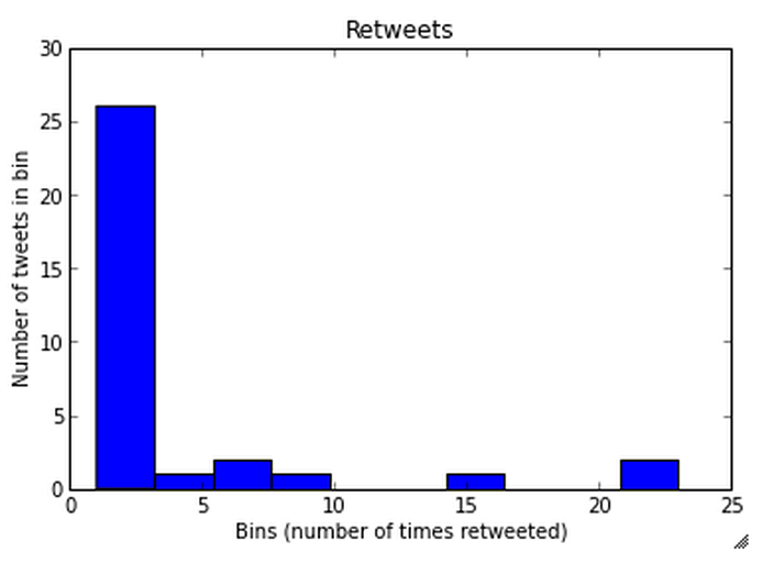
Likewise, when interpreting Figure 1.6, “A histogram of retweet frequencies”, we see that there are a select few tweets that are retweeted with a much higher frequencies than the bulk of the tweets, which are retweeted only once and account for the majority of the volume given by the largest blue rectangle on the left side of the histogram.
The code for generating these histograms directly in IPython Notebook is given in Examples 1.13 and 1.14. Taking some time to explore the capabilities of matplotlib and other scientific computing tools is a worthwhile investment.
for label, data in (('Words', words),
                    ('Screen Names', screen_names),
                    ('Hashtags', hashtags)):

    # Build a frequency map for each set of data
    # and plot the values
    c = Counter(data)
    plt.hist(c.values())

    # Add a title and y-label ...
    plt.title(label)
    plt.ylabel("Number of items in bin")
    plt.xlabel("Bins (number of times an item appeared)")

    # ... and display as a new figure
    plt.figure()
# Using underscores while unpacking values in
# a tuple is idiomatic for discarding them

counts = [count for count, _, _ in retweets]

plt.hist(counts)
plt.title("Retweets")
plt.xlabel('Bins (number of times retweeted)')
plt.ylabel('Number of tweets in bin')

print counts
This chapter introduced Twitter as a successful technology platform that has grown virally and become "all the rage," given its ability to satisfy some fundamental human desires relating to communication, curiosity, and the self-organizing behavior that has emerged from its chaotic network dynamics. The example code in this chapter got you up and running with Twitter's API, illustrated how easy (and fun) it is to use Python to interactively explore and analyze Twitter data, and provided some starting templates that you can use for mining tweets. We started out the chapter by learning how to create an authenticated connection and then progressed through a series of examples that illustrated how to discover trending topics for particular locales, how to search for tweets that might be interesting, and how to analyze those tweets using some elementary but effective techniques based on frequency analysis and simple statistics. Even what seemed like a somewhat arbitrary trending topic turned out to lead us down worthwhile paths with lots of possibilities for additional analysis.
Note:Chapter 9, Twitter Cookbook contains a number of Twitter recipes covering a broad array of topics that range from tweet harvesting and analysis to the effective use of storage for archiving tweets to techniques for analyzing followers for insights.
One of the primary takeaways from this chapter from an analytical standpoint is that counting is generally the first step to any kind of meaningful quantitative analysis. Although basic frequency analysis is simple, it is a powerful tool for your repertoire that shouldn’t be overlooked just because it’s so obvious; besides, many other advanced statistics depend on it. On the contrary, frequency analysis and measures such as lexical diversity should be employed early and often, for precisely the reason that doing so is so obvious and simple. Oftentimes, but not always, the results from the simplest techniques can rival the quality of those from more sophisticated analytics. With respect to data in the Twitterverse, these modest techniques can usually get you quite a long way toward answering the question, “What are people talking about right now?” Now that's something we'd all like to know, isn't it?
Note:The source code outlined for this chapter and all other chapters is available at GitHub in a convenient IPython Notebook format that you're highly encouraged to try out from the comfort of your own web browser.
Bookmark and spend some time reviewing Twitter's API documentation. In particular, spend some time browsing the information on the REST API and platform objects.
If you haven't already, get comfortable working in IPython and IPython Notebook as a more productive alternative to the traditional Python interpreter. Over the course of your social web mining career, the saved time and increased productivity will really start to add up.
If you have a Twitter account with a nontrivial number of tweets, request your historical tweet archive from your account settings and analyze it. The export of your account data includes files organized by time period in a convenient JSON format. See the README.txt file included in the downloaded archive for more details. What are the most common terms that appear in your tweets? Who do you retweet the most often? How many of your tweets are retweeted (and why do you think this is the case)?
Take some time to explore Twitter's REST API with its developer console. Although we opted to dive in with the twitter Python package in a programmatic fashion in this chapter, the console can be useful for exploring the API, the effects of parameters, and more. The command-line tool Twurl is another option to consider if you prefer working in a terminal.
Complete the exercise of determining whether there seems to be a spiritual or religious affiliation for the users who retweeted the status citing "God" as someone important to them, or follow the workflow in this chapter for a trending topic or arbitrary search query of your own choosing. Explore some of the advanced search features that are available for more precise querying.
Explore Yahoo! GeoPlanet's Where On Earth ID API so that you can compare and contrast trends from different locales.
Take a closer look at matplotlib and learn how to create beautiful plots of 2D and 3D data with IPython Notebook.
Explore and apply some of the exercises from Chapter 9, Twitter Cookbook.
The following list of links from this chapter may be useful for review:
[1] Although it's an implementation detail, it may be worth noting that Twitter's v1.1 API still implements OAuth 1.0a, whereas many other social web properties have since upgraded to OAuth 2.0.